Introduction介绍
On the cosmic scale, gravitation dominates the universe. Nuclear and electromagnetic forces account for the detailed processes that allow stars to shine and astronomers to see them. But it is gravitation that shapes the universe, determining the geometry of space and time and thus the large-scale distribution of galaxies. Providing insight into gravitation – its effects, its nature and its causes – is therefore rightly seen as one of the most important goals of physics and astronomy.在宇宙尺度上,引力主宰着宇宙。核力和电磁力解释了恒星发光和天文学家看到它们的详细过程。但正是引力塑造了宇宙,决定了空间和时间的几何形状,从而决定了星系的大尺度分布。因此,深入了解引力——它的影响、性质和原因——被正确地视为物理学和天文学最重要的目标之一。
Through more than a thousand years of human history the common explanation of gravitation was based on the Aristotelian belief that objects had a natural place in an Earth-centred universe that they would seek out if free to do so. For about two and a half centuries the Newtonian idea of gravity as a force held sway. Then, in the twentieth century, came Einstein’s conception of gravity as a manifestation of spacetime curvature. It is this latter view that is the main concern of this book.在一千多年的人类历史中,对万有引力的常见解释是基于亚里士多德的信念,即物体在以地球为中心的宇宙中拥有一个自然的位置,如果可以自由地这样做,它们就会寻找这个位置。大约两个半世纪以来,牛顿引力作为一种力的观念一直占据主导地位。然后,在二十世纪,爱因斯坦提出了引力作为时空曲率表现的概念。本书主要关注的正是后一种观点。
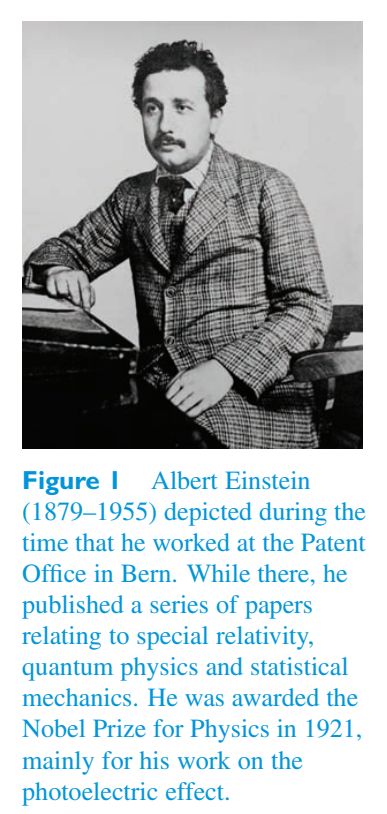
The story of Einsteinian gravitation begins with a failure. Einstein’s theory of special relativity, published in 1905 while he was working as a clerk in the Swiss Patent Office in Bern, marked an enormous step forward in theoretical physics and soon brought him academic recognition and personal fame. However, it also showed that the Newtonian idea of a gravitational force was inconsistent with the relativistic approach and that a new theory of gravitation was required. Ten years later, Einstein’s general theory of relativity met that need, highlighting the important role of geometry in accounting for gravitational phenomena and leading on to concepts such as black holes and gravitational waves. Within a year and a half of its completion, the new theory was providing the basis for a novel approach to cosmology – the science of the universe – that would soon have to take account of the astronomy of galaxies and the physics of cosmic expansion. The change in thinking demanded by relativity was radical and profound. Its mastery is one of the great challenges and greatest delights of any serious study of physical science.爱因斯坦引力的故事始于一次失败。 1905 年,爱因斯坦在伯尔尼的瑞士专利局担任职员时发表了狭义相对论,标志着理论物理学向前迈出了一大步,并很快为他带来了学术认可和个人声誉。然而,它也表明牛顿的引力思想与相对论方法不一致,需要一种新的引力理论。十年后,爱因斯坦的广义相对论满足了这一需求,强调了几何学在解释引力现象中的重要作用,并引出了黑洞和引力波等概念。在完成后的一年半内,新理论为宇宙学(宇宙科学)的新方法提供了基础,该方法很快就必须考虑星系天文学和宇宙膨胀物理学。相对论所要求的思维变革是彻底而深刻的。掌握它是任何严肃的物理科学研究的巨大挑战和最大的乐趣之一。
This book begins with two chapters devoted to special relativity. These are followed by a mainly mathematical chapter that provides the background in geometry that is needed to appreciate Einstein’s subsequent development of the theory. Chapter 4 examines the basic principles and assumptions of general relativity – Einstein’s theory of gravity – while Chapters 5 and 6 apply the theory to an isolated spherical body and then extend that analysis to non-rotating and rotating black holes. Chapter 7 concerns the testing of general relativity, including the use of astronomical observations and gravitational waves. Finally, Chapter 8 examines modern relativistic cosmology, setting the scene for further and ongoing studies of observational cosmology.本书开头有两章专门讨论狭义相对论。接下来是主要是数学的章节,提供理解爱因斯坦随后理论发展所需的几何背景。第 4 章探讨了广义相对论(爱因斯坦的引力理论)的基本原理和假设,而第 5 章和第 6 章将该理论应用于孤立的球体,然后将该分析扩展到非旋转和旋转黑洞。第七章涉及广义相对论的检验,包括天文观测和引力波的使用。最后,第八章探讨了现代相对论宇宙学,为进一步和正在进行的观测宇宙学研究奠定了基础。
The text before you is the result of a collaborative effort involving a team of authors and editors working as part of the broader effort to produce the Open University course S383 The Relativistic Universe. Details of the team’s membership and responsibilities are listed elsewhere but it is appropriate to acknowledge here the particular contributions of Jim Hague regarding Chapters 1 and 2, Derek Capper concerning Chapters 3, 4 and 7, and Aiden Droogan in relation to Chapters 5, 6 and 8. Robert Lambourne was responsible for planning and producing the final unified text which benefited greatly from the input of the S383 Course Team Chair, Andrew Norton, and the attention of production editor您面前的文本是作者和编辑团队共同努力的结果,作为制作开放大学课程 S383 相对论宇宙的更广泛努力的一部分。团队成员和职责的详细信息在其他地方列出,但在此应感谢 Jim Hague 对第 1 章和第 2 章的特殊贡献,Derek Capper 对第 3、4 和 7 章的特殊贡献,以及 Aiden Droogan 对第 5、6 和 8 章的特殊贡献。Robert Lambourne 负责规划和制作最终的统一文本,这得益于 S383 课程团队主席 Andrew Norton 的投入以及制作编辑的关注
Peter Twomey. The whole team drew heavily on the work and wisdom of an earlier Open University Course Team that was responsible for the production of the course S357 Space, Time and Cosmology.彼得·图梅.整个团队很大程度上借鉴了早期开放大学课程团队的工作和智慧,该团队负责制作 S357 空间、时间和宇宙学课程。
A major aim for this book is to allow upper-level undergraduate students to develop the skills and confidence needed to pursue the independent study of the many more comprehensive texts that are now available to students of relativity, gravitation and cosmology. To facilitate this the current text has largely adopted the notation used in the outstanding book by Hobson et al.本书的主要目的是让高年级本科生培养独立研究相对论、引力和宇宙学学生现在可以使用的许多更全面的文本所需的技能和信心。为了方便这一点,当前的文本很大程度上采用了 Hobson 等人的杰出著作中使用的符号。
General Relativity: An Introduction for Physicists, M. P. Hobson, G. Efstathiou and A. N. Lasenby, Cambridge University Press, 2006.《广义相对论:物理学家简介》,M. P. Hobson、G. Efstathiou 和 A. N. Lasenby,剑桥大学出版社,2006 年。
Other books that provide valuable further reading are (roughly in order of increasing mathematical demand):其他提供有价值的进一步阅读的书籍是(大致按照数学需求增加的顺序排列):
An Introduction to Modern Cosmology, A. Liddle, Wiley,现代宇宙学导论,A. Liddle,Wiley,
1999.1999 年。
Relativity, Gravitation and Cosmology: A Basic Introduction, T-P. Cheng, Oxford University Press: 2005. Introducing Einstein’s Relativity, R. d’Inverno, Oxford University Press, 1992. Relativity: Special, General and Cosmological, W. Rindler, Oxford University Press, 2001. Cosmology, S. Weinberg, Cambridge University Press,相对论、引力和宇宙学:基本介绍,T-P。 Cheng,牛津大学出版社:2005。介绍爱因斯坦的相对论,R. d’Inverno,牛津大学出版社,1992。相对论:狭义、广义和宇宙学,W. Rindler,牛津大学出版社,2001。宇宙学,S. Weinberg,剑桥大学出版社,
2008.2008年。
Two useful sources of reprints of original papers of historical significance are:具有历史意义的原始论文重印的两个有用来源是:
The Principle of Relativity, A. Einstein et al., Dover, New York, 1952. Cosmological Constants, edited by J. Bernstein and G. Feinberg, Columbia University Press, 1986.《相对论原理》,A. Einstein 等人,多佛,纽约,1952 年。《宇宙学常数》,J. Bernstein 和 G. Feinberg 编辑,哥伦比亚大学出版社,1986 年。
Those wishing to undertake background reading in astronomy, physics and mathematics to support their study of this book or of any of the others listed above might find the following particularly helpful:那些希望进行天文学、物理和数学背景阅读以支持他们对本书或上述任何其他书籍的研究的人可能会发现以下内容特别有帮助:
An Introduction to Galaxies and Cosmology, edited by M. H. Jones and R. J. A. Lambourne, Cambridge University Press, 2003. The seven volumes in the series The Physical World, edited by R. J. A. Lambourne, A. J. Norton et al., Institute of Physics Publishing, 2000. (Go to www.physicalworld.org for further details.) The paired volumes Basic Mathematics for the Physical Sciences, edited by R. J. A. Lambourne and M. H. Tinker, Wiley, 2000. Further Mathematics for the Physical Sciences, edited by M. H. Tinker and R. J. A. Lambourne, Wiley, 2000.《星系和宇宙学导论》,由 M. H. Jones 和 R. J. A. Lambourne 编辑,剑桥大学出版社,2003 年。《物理世界》系列的七卷,由 R. J. A. Lambourne、A. J. Norton 等人编辑,Institute of Physical Publishing,2000 年。(更多详细信息,请访问 www.physicalworld.org。) R. J. A. Lambourne 和 M. H. Tinker,Wiley,2000。《物理科学的进一步数学》,M. H. Tinker 和 R. J. A. Lambourne 编辑,Wiley,2000 年。
Chapter 1 Special relativity and spacetime第一章狭义相对论与时空
Introduction介绍
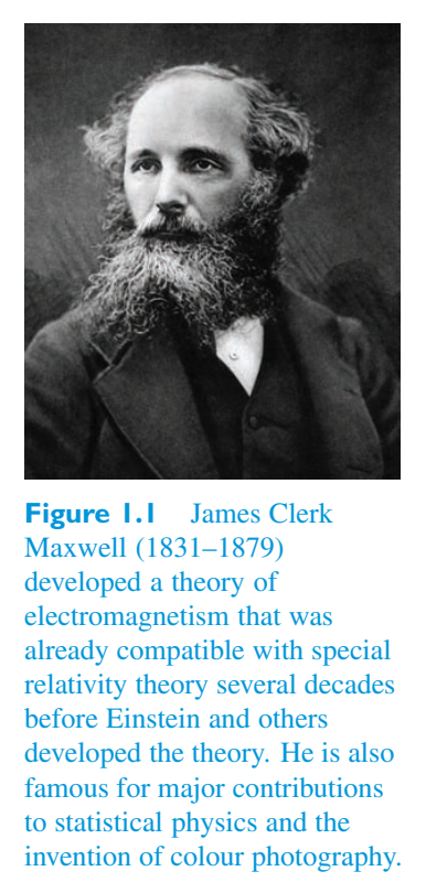
In two seminal papers in 1861 and 1864, and in his treatise of 1873, James Clerk Maxwell (Figure 1.1), Scottish physicist and genius, wrote down his revolutionary unified theory of electricity and magnetism, a theory that is now summarized in the equations that bear his name. One of the deep results of the theory introduced by Maxwell was the prediction that wave-like excitations of combined electric and magnetic fields would travel through a vacuum with the same speed as light. It was soon widely accepted that light itself was an electromagnetic disturbance propagating through space, thus unifying electricity and magnetism with optics.苏格兰物理学家和天才詹姆斯·克拉克·麦克斯韦(James Clerk Maxwell)(图 1.1)在 1861 年和 1864 年的两篇开创性论文以及 1873 年的论文中写下了他革命性的电学和磁学统一理论,该理论现在被总结为以他的名字命名的方程。麦克斯韦提出的理论的深刻成果之一是预测电场和磁场组合的波状激发将以与光速相同的速度穿过真空。很快人们就广泛接受光本身是一种通过空间传播的电磁扰动,从而将电、磁与光学统一起来。
The fundamental work of Maxwell opened the way for an understanding of the universe at a much deeper level. Maxwell himself, in common with many scientists of the nineteenth century, believed in an all-pervading medium called the ether, through which electromagnetic disturbances travelled, just as ocean waves travelled through water. Maxwell’s theory predicted that light travels with the same speed in all directions, so it was generally assumed that the theory predicted the results of measurements made using equipment that was at rest with respect to the ether. Since the Earth was expected to move through the ether as it orbited the Sun, measurements made in terrestrial laboratories were expected to show that light actually travelled with different speeds in different directions, allowing the speed of the Earth’s movement through the ether to be determined.麦克斯韦的基础工作为更深层次地理解宇宙开辟了道路。麦克斯韦本人与 19 世纪的许多科学家一样,相信有一种称为以太的无所不在的介质,电磁扰动通过它传播,就像海浪在水中传播一样。麦克斯韦理论预测光以相同的速度向各个方向传播,因此人们普遍认为该理论预测了使用相对于以太静止的设备进行的测量结果。由于预计地球绕太阳运行时会穿过以太,因此地面实验室进行的测量预计会表明光实际上以不同的速度向不同方向传播,从而可以确定地球穿过以太的运动速度。
However, the failure to detect any variations in the measured speed of light, most notably by A. A. Michelson and E. W. Morley in 1887, prompted some to suspect that measurements of the speed of light in a vacuum would always yield the same result irrespective of the motion of the measuring equipment. Explaining how this could be the case was a major challenge that prompted ingenious proposals from mathematicians and physicists such as Henri Poincaré, George Fitzgerald and Hendrik Lorentz. However, it was the young Albert Einstein who first put forward a coherent and comprehensive solution in his 1905 paper ‘On the electrodynamics of moving bodies’, which introduced the special theory of relativity. With the benefit of hindsight, we now realize that Maxwell had formulated the first major theory that was consistent with special relativity, a revolutionary new way of thinking about space and time.然而,未能检测到所测量的光速的任何变化,尤其是 1887 年 A. A. 迈克尔逊和 E. W. 莫利的测量,促使一些人怀疑真空中光速的测量总是会产生相同的结果,而与测量设备的运动无关。解释为什么会出现这种情况是一项重大挑战,促使亨利·庞加莱、乔治·菲茨杰拉德和亨德里克·洛伦兹等数学家和物理学家提出了巧妙的建议。然而,年轻的阿尔伯特·爱因斯坦在他1905年的论文《论运动物体的电动力学》中首先提出了一个连贯且全面的解决方案,该论文引入了狭义相对论。事后看来,我们现在意识到麦克斯韦提出了第一个与狭义相对论相一致的主要理论,这是一种革命性的思考空间和时间的新方式。
This chapter reviews the implications of special relativity theory for the understanding of space and time. The narrative covers the fundamentals of the theory, concentrating on some of the major differences between our intuition about space and time and the predictions of special relativity. By the end of this chapter, you should have a broad conceptual understanding of special relativity, and be able to derive its basic equations, the Lorentz transformations, from the postulates of special relativity. You will understand how to use events and intervals to describe properties of space and time far from gravitating bodies. You will also have been introduced to Minkowski spacetime, a four-dimensional fusion of space and time that provides the natural setting for discussions of special relativity.本章回顾狭义相对论对于理解空间和时间的意义。叙述涵盖理论基础,重点讨论我们关于空间和时间的直觉与狭义相对论预言之间的一些主要差异。读完本章后,你应当对狭义相对论有宽泛的概念性理解,并能够从狭义相对论的公设推导出它的基本方程,即洛伦兹变换。你将理解如何用事件和间隔来描述远离引力体处的空间和时间性质。你还会接触到闵可夫斯基时空,即空间与时间的四维融合,它为讨论狭义相对论提供了自然背景。
1.1 Basic concepts of special relativity1.1 狭义相对论的基本概念
1.1.1 Events, frames of reference and observers1.1.1 事件、参照系和观察者
When dealing with special relativity it is important to use language very precisely in order to avoid confusion and error. Fundamental to the precise description of physical phenomena is the concept of an event, the spacetime analogue of a point in space or an instant in time.在处理狭义相对论时,非常精确地使用语言以避免混淆和错误非常重要。精确描述物理现象的基础是事件的概念,即空间中的一点或时间中的瞬间的时空模拟。
Events事件
An event is an instantaneous occurrence at a specific point in space.事件是在空间中特定点瞬时发生的事件。
An exploding firecracker or a small light that flashes once are good approximations to events, since each happens at a definite time and at a definite position.爆炸的鞭炮或闪烁一次的小光都是对事件的很好的近似,因为每一个事件都发生在确定的时间和确定的位置。
To know when and where an event happened, we need to assign some coordinates to it: a time coordinate t and an ordered set of spatial coordinates such as the Cartesian coordinates (x, y, z), though we might equally well use spherical coordinates (r, \(\theta\), \(\phi\)) or any other suitable set. The important point is that we should be able to assign a unique set of clearly defined coordinates to any event. This leads us to our second important concept, a frame of reference.要知道事件发生的时间和地点,我们需要为其分配一些坐标:时间坐标 t 和一组有序的空间坐标,例如笛卡尔坐标 (x, y, z),尽管我们同样可以使用球坐标 (r, \(\theta\), \(\phi\)) 或任何其他合适的集合。重要的一点是,我们应该能够为任何事件分配一组唯一的、明确定义的坐标。这引出了我们的第二个重要概念,即参考系。
Frames of reference参考系
A frame of reference is a system for assigning coordinates to events. It consists of a system of synchronized clocks that allows a unique value of the time to be assigned to any event, and a system of spatial coordinates that allows a unique position to be assigned to any event.参考系是为事件分配坐标的系统。它由一个同步时钟系统和一个空间坐标系统组成,同步时钟系统允许为任何事件分配唯一的时间值,而空间坐标系统允许为任何事件分配唯一的位置。
In much of what follows we shall make use of a Cartesian coordinate system with axes labelled x, y and z. The precise specification of such a system involves selecting an origin and specifying the orientation of the three orthogonal axes that meet at the origin. As far as the system of clocks is concerned, you can imagine that space is filled with identical synchronized clocks all ticking together (we shall need to say more about how this might be achieved later). When using a particular frame of reference, the time assigned to an event is the time shown on the clock at the site of the event when the event happens. It is particularly important to note that the time of an event is not the time at which the event is seen at some far off point — it is the time at the event itself that matters.在接下来的大部分内容中,我们将使用笛卡尔坐标系,其轴标记为 x、y 和 z。这种系统的精确规范涉及选择原点并指定在原点相交的三个正交轴的方向。就时钟系统而言,您可以想象空间中充满了相同的同步时钟,所有这些时钟都一起滴答作响(稍后我们将需要更多地讨论如何实现这一点)。当使用特定参考系时,分配给事件的时间是事件发生时事件现场的时钟上显示的时间。特别重要的是要注意,事件发生的时间并不是在某个遥远的地方看到该事件的时间——重要的是事件本身的时间。
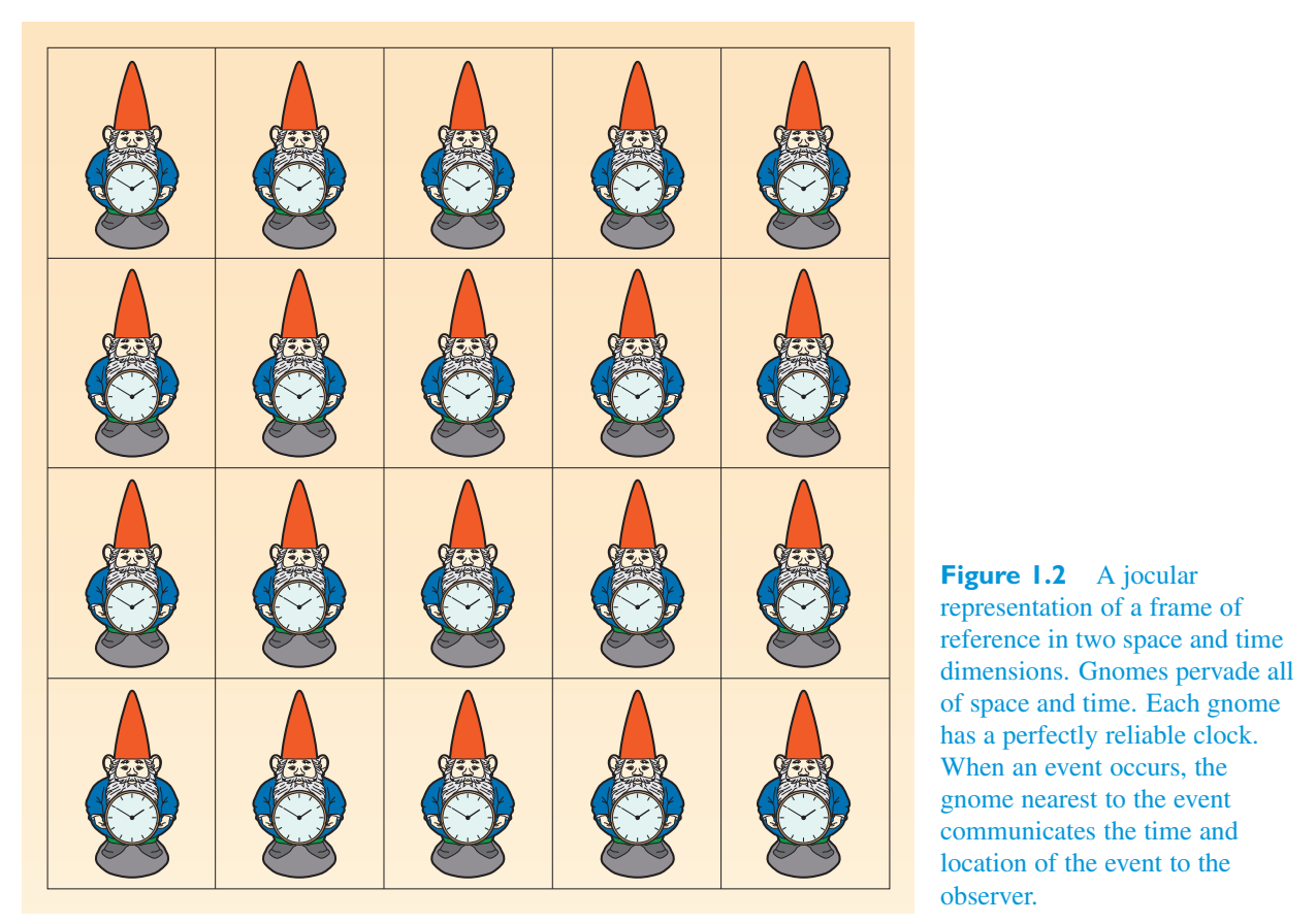
Reference frames are often represented by the letter S. Figure 1.2 provides what we hope is a memorable illustration of the basic idea, in this case with just two spatial dimensions. This might be called the frame S gnome.参考系通常用字母 S 表示。图 1.2 提供了我们希望的基本思想的令人难忘的说明,在本例中只有两个空间维度。这可能被称为框架 S 侏儒。
Among all the frames of reference that might be imagined, there is a class of frames that is particularly important in special relativity. This is the class of inertial frames. An inertial frame of reference is one in which a body that is not subject to any net force maintains a constant velocity. Equivalently, we can say the following.在所有可能想象到的参考系中,有一类参考系在狭义相对论中特别重要。这是一类惯性系。惯性参考系是指不受任何净力作用的物体保持恒定速度的参考系。同样,我们可以说如下。
Inertial frames of reference惯性参考系
An inertial frame of reference is a frame of reference in which Newton’s first law of motion holds true.惯性参考系是牛顿第一运动定律成立的参考系。
Any frame that moves with constant velocity relative to an inertial frame will also be an inertial frame. So, if you can identify or establish one inertial frame, then you can find an infinite number of such frames each having a constant velocity relative to any of the others. Any frame that accelerates relative to an inertial frame cannot be an inertial frame. Since rotation involves changing velocity, any frame that rotates relative to an inertial frame is also disqualified from being inertial.任何相对于惯性系以匀速运动的坐标系也将是惯性系。因此,如果您可以识别或建立一个惯性系,那么您就可以找到无数个这样的框架,每个框架相对于任何其他框架都具有恒定的速度。任何相对于惯性系加速的坐标系都不能是惯性系。由于旋转涉及速度的变化,因此任何相对于惯性系旋转的坐标系也被取消惯性系的资格。
One other concept is needed to complete the basic vocabulary of special relativity. This is the idea of an observer.需要另一个概念来完成狭义相对论的基本词汇。这是观察者的想法。
Observers观察者
An observer is an individual dedicated to using a particular frame of reference for recording events.观察者是致力于使用特定参考系来记录事件的个人。
We might speak of an observer O using frame S, or a different observer \(O'\) (read as ‘O-prime’) using frame \(S'\) (read as ‘S-prime’).我们可能会说一个使用框架 S 的观察者 O,或者使用框架 \(S'\)(读作“S-素数”)的不同观察者 \(O'\)(读作“O-素数”)。
Though you may think of an observer as a person, just like you or me, at rest in their chosen frame of reference, it is important to realize that an observer’s location is of no importance for reporting the coordinates of events in special relativity. The position that an observer assigns to an event is the place where it happened. The time that an observer assigns is the time that would be shown on a clock at the site of the event when the event actually happened, and where the clock concerned is part of the network of synchronized clocks always used in that observer’s frame of reference. An observer might see the explosion of a distant star tonight, but would report the time of the explosion as the time long ago when the explosion actually occurred, not the time at which the light from the explosion reached the observer’s location. To this extent, ‘seeing’ and ‘observing’ are very different processes. It is best to avoid phrases such as ‘an observer sees... ’ unless that is what you really mean. An observer measures and observes.尽管您可能将观察者视为一个人,就像您或我一样,在他们选择的参考系中休息,但重要的是要认识到观察者的位置对于报告狭义相对论中事件的坐标并不重要。观察者为事件指定的位置就是事件发生的地点。观察者分配的时间是事件实际发生时事件现场的时钟上显示的时间,并且相关时钟是始终在该观察者的参考系中使用的同步时钟网络的一部分。观察者今晚可能会看到一颗遥远恒星的爆炸,但会将爆炸时间报告为很久以前爆炸实际发生的时间,而不是爆炸发出的光到达观察者位置的时间。从这个意义上说,“看”和“观察”是非常不同的过程。最好避免使用诸如“观察者看到……”之类的短语,除非这就是您真正的意思。观察者进行测量和观察。
Any observer who uses an inertial frame of reference is said to be an inertial observer. Einstein’s special theory of relativity is mainly concerned with observations made by inertial observers. That’s why it’s called special relativity — the term ‘special’ is used in the sense of ‘restricted’ or ‘limited’. We shall not really get away from this limitation until we turn to general relativity in Chapter 4.任何使用惯性参考系的观察者都被称为惯性观察者。爱因斯坦的狭义相对论主要涉及惯性观察者的观察。这就是为什么它被称为狭义相对论——“特殊”一词的意思是“受限”或“有限”。直到我们在第四章转向广义相对论之前,我们才能真正摆脱这个限制。
Exercise 1.1 For many purposes, a frame of reference练习 1.1 出于多种目的,参考系
fixed in a laboratory on the Earth provides a good approximation to an inertial frame. However, such a frame is not really an inertial frame. How might its true, non-inertial, nature be revealed experimentally, at least in principle?固定在地球上的实验室中,可以很好地近似惯性系。然而,这样的框架并不是真正的惯性系。其真实的、非惯性的性质如何通过实验(至少在原则上)得以揭示?
1.1.2 The postulates of special relativity1.1.2 狭义相对论的假设
Physicists generally treat the laws of physics as though they hold true everywhere and at all times. There is some evidence to support such an assumption, though it is recognized as a hypothesis that might fail under extreme conditions. To the extent that the assumption is true, it does not matter where or when observations are made to test the laws of physics since the time and place of a test of fundamental laws should not have any influence on its outcome.物理学家通常认为物理定律在任何地方、任何时候都适用。有一些证据支持这种假设,尽管它被认为是在极端条件下可能失败的假设。如果假设是正确的,那么在何时何地进行观察来检验物理定律并不重要,因为基本定律检验的时间和地点不应对其结果产生任何影响。
Where and when laws are tested might not influence the outcome, but what about motion? We know that inertial and non-inertial observers will not agree about Newton’s first law. But what about different inertial observers in uniform relative motion where one observer moves at constant velocity with respect to the other? A pair of inertial observers would agree about Newton’s first law; might they also agree about other laws of physics?法律的检验地点和时间可能不会影响结果,但是运动呢?我们知道惯性和非惯性观察者不会同意牛顿第一定律。但是,当一个观察者相对于另一个观察者以恒定速度移动时,处于匀速相对运动的不同惯性观察者又会怎样呢?一对惯性观察者会同意牛顿第一定律;他们是否也同意其他物理定律?
It has long been thought that they would at least agree about the laws of mechanics. Even before Newton’s laws were formulated, the great Italian physicist Galileo Galilei (1564–1642) pointed out that a traveller on a smoothly moving boat had exactly the same experiences as someone standing on the shore. A ball game could be played on a uniformly moving ship just as well as it could be played on shore. To the early investigators, uniform motion alone appeared to have no detectable consequences as far as the laws of mechanics were concerned. An observer shut up in a sealed box that prevented any observation of the outside world would be unable to perform any mechanics experiment that would reveal the uniform velocity of the box, even though any acceleration could be easily detected. (We are all familiar with the feeling of being pressed back in our seats when a train or car accelerates forward.) These notions provided the basis for the first theory of relativity, which is now known as Galilean relativity in honour of Galileo’s original insight. This theory of relativity assumes that all inertial observers will agree about the laws of Newtonian mechanics.长期以来人们一直认为他们至少会同意力学定律。甚至在牛顿定律制定之前,伟大的意大利物理学家伽利略·伽利雷(Galileo Galilei,1564-1642)就指出,在平稳移动的船上的旅行者与站在岸上的人有着完全相同的经历。球类运动可以在均匀移动的船上进行,就像在岸上进行一样。对于早期的研究人员来说,就力学定律而言,仅匀速运动似乎没有可察觉的后果。一个观察者被关在一个无法观察外界的密封盒子里,将无法进行任何揭示盒子匀速的力学实验,即使任何加速度都可以很容易地检测到。(我们都熟悉当火车或汽车加速前进时被压在座位上的感觉。)这些概念为第一个相对论提供了基础,该理论现在被称为伽利略相对论,以纪念伽利略的原始见解。这种相对论假设所有惯性观察者都同意牛顿力学定律。
Einstein believed that inertial observers would agree about the laws of physics quite generally, not just in mechanics. But he was not convinced that Galilean relativity was correct, which brought Newtonian mechanics into question. The only statement that he wanted to presume as a law of physics was that all inertial observers agreed about the speed of light in a vacuum. Starting from this minimal assumption, Einstein was led to a new theory of relativity that was markedly different from Galilean relativity. The new theory, the special theory of relativity, supported Maxwell’s laws of electromagnetism but caused the laws of mechanics to be substantially rewritten. It also provided extraordinary new insights into space and time that will occupy us for the rest of this chapter.爱因斯坦相信,惯性观察者会普遍同意物理定律,而不仅仅是力学方面的。但他不相信伽利略相对论是正确的,这使牛顿力学受到质疑。他想假定为物理定律的唯一陈述是所有惯性观察者都同意真空中的光速。从这个最小的假设出发,爱因斯坦提出了一种与伽利略相对论明显不同的新相对论。新理论,即狭义相对论,支持麦克斯韦电磁定律,但导致力学定律被大幅改写。它还提供了对空间和时间的非同寻常的新见解,这将占据我们本章余下的部分。
Einstein based the special theory of relativity on two postulates, that is, two statements that he believed to be true on the basis of the physics that he knew. The first postulate is often referred to as the principle of relativity.爱因斯坦将狭义相对论建立在两个假设的基础上,也就是说,他根据他所知道的物理学相信这两个陈述是正确的。第一个假设通常被称为相对性原理。
The first postulate of special relativity狭义相对论第一公设
The laws of physics can be written in the same form in all inertial frames.物理定律可以在所有惯性系中以相同的形式书写。
This is a bold extension of the earlier belief that observers would agree about the laws of mechanics, but it is not at first sight exceptionally outrageous. It will, however, have profound consequences.这是对早期观点的大胆延伸,即观察者会同意力学定律,但乍一看这并不是特别离谱。然而,这将产生深远的影响。
The second postulate is the one that gives primacy to the behaviour of light, a subject that was already known as a source of difficulty. This postulate is sometimes referred to as the principle of the constancy of the speed of light.第二个假设将光的行为置于首要地位,这是一个众所周知的困难来源的主题。该假设有时被称为光速恒定原理。
The second postulate of special relativity狭义相对论第二公设
The speed of light in a vacuum has the same constant value, c = \(3\times10^{8}\) \(\mathrm{m\,s^{-1}}\), in all inertial frames.在所有惯性系中,真空中的光速具有相同的常数值,c = \(3\times10^{8}\) \(\mathrm{m\,s^{-1}}\)。
This postulate certainly accounts for Michelson and Morley’s failure to detect any variations in the speed of light, but at first sight it still seems crazy. Our experience with everyday objects moving at speeds that are small compared with the speed of light tells us that if someone in a car that is travelling forward at speed v throws something forward at speed w relative to the car, then, according to an observer standing on the roadside, the thrown object will move forward with speed v + w. But the second postulate tells us that if the traveller in the car turns on a torch, effectively throwing forward some light moving at speed c relative to the car, then the roadside observer will also find that the light travels at speed c, not the v + c that might have been expected. Einstein realized that for this to be true, space and time must behave in previously unexpected ways.这个假设当然可以解释迈克尔逊和莫利未能检测到光速的任何变化,但乍一看它仍然看起来很疯狂。我们对日常物体以小于光速的速度运动的经验告诉我们,如果一辆以速度 v 向前行驶的汽车中的某个人以相对于汽车的速度 w 向前扔东西,那么,根据站在路边的观察者的说法,扔出的物体将以速度 v + w 向前移动。但第二个假设告诉我们,如果车里的旅行者打开手电筒,有效地向前投射一些相对于汽车以 c 速度移动的光,那么路边观察者也会发现光以 c 速度传播,而不是预期的 v + c 速度。爱因斯坦意识到,要实现这一点,空间和时间必须以以前意想不到的方式运行。
The second postulate has another important consequence. Since all observers agree about the speed of light, it is possible to use light signals (or any other electromagnetic signal that travels at the speed of light) to ensure that the network of clocks we imagine each observer to be using is properly synchronized. We shall not go into the details of how this is done, but it is worth pointing out that if an observer sent a radar signal (which travels at the speed of light) so that it arrived at an event just as the event was happening and was immediately reflected back, then the time of the event would be midway between the times of transmission and reception of the radar signal. Similarly, the distance to the event would be given by half the round trip travel time of the signal, multiplied by the speed of light.第二个假设还有另一个重要的结果。由于所有观察者都同意光速,因此可以使用光信号(或以光速传播的任何其他电磁信号)来确保我们想象的每个观察者使用的时钟网络正确同步。我们不会详细说明这是如何完成的,但值得指出的是,如果观察者发送雷达信号(以光速传播),使其在事件发生时到达事件并立即反射回来,那么事件发生的时间将介于雷达信号的传输时间和接收时间之间。类似地,到事件的距离将由信号往返传播时间的一半乘以光速得出。
1.2 Coordinate transformations1.2 坐标变换
A theory of relativity concerns the relationship between observations made by observers in relative motion. In the case of special relativity, the observers will be inertial observers in uniform relative motion, and their most fundamental observations will be the time and space coordinates of events.相对论涉及观察者在相对运动中所做的观察之间的关系。在狭义相对论中,观察者将是匀速相对运动的惯性观察者,他们最基本的观察将是事件的时间和空间坐标。
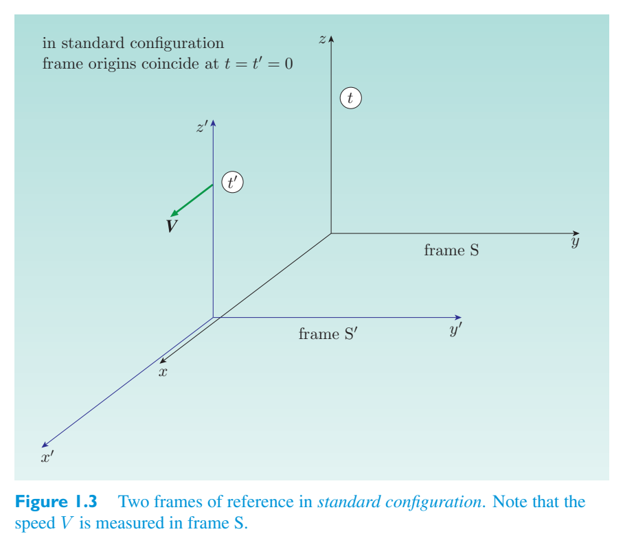
For the sake of definiteness and simplicity, we shall consider two inertial observers O and \(O'\) whose respective frames of reference, S and \(S'\), are arranged in the following standard configuration (see Figure 1.3):为了明确和简单起见,我们考虑两个惯性观测器 O 和 \(O'\),其各自的参考系 S 和 \(S'\) 按以下标准配置排列(见图 1.3):
1. The origin of frame \(S'\) moves along the x -axis of1. 坐标系\(S'\)的原点沿x轴移动
frame S, in the direction of increasing values of x, with constant velocity V as measured in S.坐标系 S,沿 x 值增加的方向,具有在 S 中测量的恒定速度 V。
2. The x -, y - and z -axes of frame S are always parallel2. 框架S的x、y、z轴始终平行
to the corresponding \(x'\)-, \(y'\)- and \(z'\)-axes of frame \(S'\).到框架 \(S'\) 相应的 \(x'\)-、\(y'\)- 和 \(z'\)- 轴。
3. The event at which the origins of S and \(S'\) coincide3. S与\(S'\)的起源重合的事件
occurs at time t = 0 in frame S and at time \(t'\) = 0 in frame \(S'\).发生在帧 S 中的时间 t = 0 处以及帧 \(S'\) 中的时间 \(t'\) = 0 处。
We shall make extensive use of ‘standard configuration’ in what follows. The arrangement does not entail any real loss of generality since any pair of inertial frames in uniform relative motion can be placed in standard configuration by choosing to reorientate the coordinate axes in an appropriate way and by resetting the clocks appropriately.下面我们将大量使用“标准配置”。该布置不会造成任何真正的通用性损失,因为通过选择以适当的方式重新定向坐标轴并通过适当地重置时钟,可以将任何一对匀速相对运动的惯性系置于标准配置中。
In general, the observers using the frames S and \(S'\) will not agree about the coordinates of an event, but since each observer is using a well-defined frame of coordinates (t, x, y, z) reference, there must exist a set of equations relating the assigned to a particular event by observer O, to the coordinates assigned to the same event by observer \(O'\). The set of equations that performs the task of relating the two sets of coordinates is called a coordinate transformation. This section considers first the Galilean transformations that provide the basis of Galilean relativity, and then the Lorentz transformations on which Einstein’s special relativity is based.一般来说,使用坐标系 S 和 \(S'\) 的观察者不会就事件的坐标达成一致,但由于每个观察者都使用明确定义的坐标系 (t, x, y, z) 参考,因此必须存在一组方程,将观察者 O 分配给特定事件的坐标与观察者 \(O'\) 分配给同一事件的坐标相关联。执行关联两组坐标任务的方程组称为坐标变换。本节首先考虑提供伽利略相对论基础的伽利略变换,然后考虑爱因斯坦狭义相对论所基于的洛伦兹变换。
1.2.1 The Galilean transformations1.2.1 伽利略变换
Before the introduction of special relativity, most physicists would have said that the coordinate transformation between S and \(S'\) was ‘obvious’, and they would have written down the following Galilean transformations:在引入狭义相对论之前,大多数物理学家都会说S和\(S'\)之间的坐标变换是“显而易见的”,他们会写下以下伽利略变换:
where V = | V | is the relative speed of \(S'\) with respect to S.其中 V = | V |是 \(S'\) 相对于 S 的相对速度。
1.2.2 The Lorentz transformations1.2.2 洛伦兹变换
Rather than rely on intuition and run the risk of making unjustified assumptions, Einstein chose to set out his two postulates and use them to deduce the appropriate coordinate transformation between S and \(S'\). A derivation will be given later, but before that let’s examine the result that Einstein found. The equations that he derived had already been obtained by the Dutch physicist Hendrik Lorentz (Figure 1.4) in the course of his own investigations into light and electromagnetism. For that reason, they are known as the Lorentz transformations even though Lorentz did not interpret or utilize them in the same way that Einstein did. Here are the equations:爱因斯坦没有依靠直觉并冒着做出不合理假设的风险,而是选择提出他的两个假设并用它们来推导出 S 和 \(S'\) 之间适当的坐标变换。稍后将给出推导,但在此之前我们先来看看爱因斯坦发现的结果。他推导出来的方程已经由荷兰物理学家亨德里克·洛伦兹(图 1.4)在他自己对光和电磁学的研究过程中获得。因此,它们被称为洛伦兹变换,尽管洛伦兹并没有像爱因斯坦那样解释或利用它们。以下是方程式:
It is clear that the Lorentz transformations are very different from the Galilean transformations. They indicate a thorough mixing together of space and time, since the \(t'\)-coordinate of an event now depends on both t and x, just as the \(x'\)-coordinate does. According to the Lorentz transformations, the two observers do not generally agree about the time of events, even though they still agree about the time at which the origins of their respective frames coincided. So, time is no longer an absolute quantity that all observers agree about. To be meaningful, statements about the time of an event must now be associated with a particular observer. Also, the extent to which the observers - disagree about the position of an event has been modified by a factor of 1/1 − \(V^{2}\)/\(c^2\). In fact, this multiplicative factor is so common in special relativity that it is usually referred to as the the symbol \(\gamma(V)\), Lorentz factor or gamma factor and is represented by emphasizing that its value depends on the relative speed V of the two frames. Using this factor, the Lorentz transformations can be written in the following compact form.显然,洛伦兹变换与伽利略变换有很大不同。它们表明空间和时间的彻底混合,因为事件的 \(t'\) 坐标现在取决于 t 和 x,就像 \(x'\) 坐标一样。根据洛伦兹变换,两个观察者对于事件发生的时间总体上并不达成一致,尽管他们仍然同意各自框架的起源重合的时间。因此,时间不再是所有观察者都同意的绝对量。为了有意义,有关事件时间的陈述现在必须与特定的观察者相关联。此外,观察者对事件位置的分歧程度已按 1/1 系数修改 - \(V^{2}\)/\(c^2\)。事实上,这个乘法因子在狭义相对论中非常常见,通常被称为符号 \(\gamma(V)\)、洛伦兹因子或伽马因子,并通过强调其值取决于两个框架的相对速度 V 来表示。使用这个因子,洛伦兹变换可以写成以下紧凑的形式。
The Lorentz transformations洛伦兹变换
where在哪里
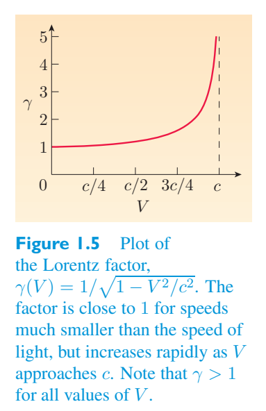
Figure 1.5 shows how the Lorentz factor grows as the relative speed V of the two frames increases. For speeds that are small compared with the speed of light, \(\gamma(V)\) ≈ 1, and the Lorentz transformations approximate the Galilean transformations provided that x is not too large. As the relative speed of the two frames approaches the speed of light, however, the Lorentz factor grows rapidly and so do the discrepancies between the Galilean and Lorentz transformations.图 1.5 显示了洛伦兹因子如何随着两坐标系相对速度 V 的增加而增长。对于与光速相比较小的速度,\(\gamma(V)\) ≈ 1,并且洛伦兹变换近似于伽利略变换,前提是 x 不太大。然而,当两个框架的相对速度接近光速时,洛伦兹因子迅速增长,伽利略变换和洛伦兹变换之间的差异也随之增大。
Exercise 1.2 Compute the Lorentz factor \(\gamma(V)\) when the relative speed V is练习1.2 计算相对速度V为时的洛伦兹因子γ(V)
(a) 10% of the speed of light, and (b) 90% of the speed of light.(a) 10% 光速,(b) 90% 光速。
The Lorentz transformations are so important in special relativity that you will see them written in many different ways. They are often presented in matrix form, as洛伦兹变换在狭义相对论中非常重要,您会看到它们以多种不同的方式书写。它们通常以矩阵形式呈现,如
You should convince yourself that this matrix multiplication gives equations equivalent to the Lorentz transformations. (The equation for transforming the time coordinate is multiplied by c.) We can also represent this relationship by the equation您应该说服自己,该矩阵乘法给出的方程相当于洛伦兹变换。 (时间坐标变换方程乘以c。)我们也可以用方程来表示这种关系
where we use the symbol \([x^{\mu}]\) to represent the column vector with components (\(x^0\), \(x^1\), \(x_{2}\), \(x^{3}\)) = (ct, x, y, z), and the symbol [\(\Lambda\) \(\mu\)] to represent the Lorentz transformation matrix其中我们使用符号 \([x^{\mu}]\) 表示分量为 (\(x^0\), \(x^1\), \(x_{2}\), \(x^{3}\)) = (ct, x, y, z) 的列向量,并使用符号 [\(\Lambda\) \(\mu\)] 表示洛伦兹变换矩阵
At this stage, when dealing with an individual matrix element \(\Lambda\) \(\mu\) \(\nu\), you can simply regard the first index as indicating the row to which it belongs and the second index as indicating the column. It then makes sense that each of the elements x \(\mu\) in the column vector \([x^{\mu}]\) should have a raised index. However, as you will see later, in the context of relativity the positioning of these indices actually has a much greater significance.此时,在处理单个矩阵元素 \(\Lambda\) \(\mu\) \(\nu\) 时,可以简单地将第一个索引视为表示其所属的行,第二个索引表示其所属的列。那么,列向量 \([x^{\mu}]\) 中的每个元素 x \(\mu\) 应该具有升高的索引,这是有意义的。然而,正如您稍后将看到的,在相对论的背景下,这些指数的定位实际上具有更大的意义。
The quantity \([x^{\mu}]\) is sometimes called the four-position since its four components (ct, x, y, z) describe the position of the event in time and space. Note that by using ct to convey the time information, rather than just t, all four components of the four-position are measured in units of distance. Also note that the Greek indices \(\mu\) and \(\nu\) take the values 0 to 3. It is conventional in special and general relativity to start the indexing of the vectors and matrices from zero, where \(x^0\) = ct. This is because the time coordinate has special properties.量 \([x^{\mu}]\) 有时称为四位置,因为它的四个分量 (ct、x、y、z) 描述了事件在时间和空间中的位置。请注意,通过使用 ct 而不仅仅是 t 来传达时间信息,四位置的所有四个分量均以距离为单位进行测量。另请注意,希腊指数 \(\mu\) 和 \(\nu\) 的值为 0 到 3。在狭义相对论和广义相对论中,通常从零开始对向量和矩阵进行索引,其中 \(x^0\) = ct。这是因为时间坐标具有特殊的属性。
Using the individual components of the four-position, another way of writing the Lorentz transformation is in terms of summations:使用四位的各个分量,洛伦兹变换的另一种编写方式是求和:
This one line really represents four different equations, one for each value of \(\mu\). When an index is used in this way, it is said to be a free index, since we are free to give it any value between 0 and 3, and whatever choice we make indicates a different equation. The index \(\nu\) that appears in the summation is not free, since whatever value we choose for \(\mu\), we are required to sum over all possible values of \(\nu\) to obtain the final equation. This means that we could replace all appearances of \(\nu\) by some other index, \(\alpha\) say, without actually changing anything. An index that is summed over in this way is said to be a dummy index.这一行实际上代表了四个不同的方程,每个方程对应 \(\mu\) 的每个值。当以这种方式使用索引时,它被称为自由索引,因为我们可以自由地给它提供 0 到 3 之间的任何值,并且无论我们做出什么选择都表示不同的方程。求和中出现的索引 \(\nu\) 不是自由的,因为无论我们为 \(\mu\) 选择什么值,我们都需要对 \(\nu\) 的所有可能值求和以获得最终方程。这意味着我们可以用其他索引(例如 \(\alpha\))替换 \(\nu\) 的所有外观,而无需实际更改任何内容。以这种方式求和的索引被称为虚拟索引。
Familiarity with the summation form of the Lorentz transformations is particularly useful when beginning the discussion of general relativity; you will meet many such sums. Before moving on, you should convince yourself that you can easily switch between the use of separate equations, matrices (including the use of four-positions) and summations when representing Lorentz transformations.在开始讨论广义相对论时,熟悉洛伦兹变换的求和形式特别有用。你会遇到很多这样的金额。在继续之前,您应该说服自己,在表示洛伦兹变换时,您可以轻松地在使用单独的方程、矩阵(包括使用四位)和求和之间切换。
Given the coordinates of an event in frame S, the Lorentz transformations tell us the coordinates of that same event as observed in frame \(S'\). It is equally important that there is some way to transform coordinates in frame \(S'\) back into the coordinates in frame S. The transformations that perform this task are known as the inverse Lorentz transformations.给定帧 S 中事件的坐标,洛伦兹变换告诉我们在帧 \(S'\) 中观察到的同一事件的坐标。同样重要的是,有某种方法可以将框架 \(S'\) 中的坐标变换回框架 S 中的坐标。执行此任务的变换称为洛伦兹逆变换。
The inverse Lorentz transformations洛伦兹逆变换
Note that the only difference between the Lorentz transformations and their inverses is that all the primed and unprimed quantities have been interchanged, and the relative speed of the two frames, V, has been replaced by the quantity − V. (This changes the transformations but not the value of the write that as \(\gamma(V)\).) Lorentz factor, which depends only on \(V^{2}\), so we can still This relationship between the transformations is expected, since frame \(S'\) is moving with speed V in the positive x -direction as measured in frame S, while frame S is moving with speed V in the negative \(x'\)-direction as measured in frame \(S'\). You should confirm that performing a Lorentz transformation and its inverse transformation in succession really does lead back to the original coordinates, i.e. (ct, x, y, z) → (\(ct'\), \(x'\), \(y'\), \(z'\)) → (ct, x, y, z).请注意,洛伦兹变换及其逆变换之间的唯一区别在于,所有启动和未启动的量都已互换,并且两个框架的相对速度 V 已被量 - V 取代。(这会改变变换,但不会改变写入的值,如 \(\gamma(V)\)。)洛伦兹因子,仅取决于 \(V^{2}\),因此我们仍然可以预期变换之间的这种关系,因为帧 \(S'\) 在帧 S 中测量的正 x 方向上以速度 V 移动,而帧 S 帧 S 中测量的负 \(x'\) 方向上以速度 V 移动AAAQQ4ZZZ。您应该确认连续执行洛伦兹变换及其逆变换确实会返回原始坐标,即 (ct, x, y, z) → (\(ct'\), \(x'\), \(y'\), \(z'\)) → (ct, x, y, z)。
- ● An event occurs at coordinates (ct = 3 m, x = 4 m● 事件发生在坐标 (ct = 3 m, x = 4 m
, y = 0, z = 0) in frame S according to an observer O. What are the coordinates of the same with speed V = 3 c/4 event in frame \(S'\) according to an observer \(O'\), moving in the positive x -direction, as measured in S?,y = 0,z = 0),根据观察者 O,在坐标系 S 中。根据观察者 \(O'\),在坐标系 \(S'\) 中,速度 V = 3 c/4 的相同事件的坐标是多少,在 S 中测量,沿正 x 方向移动?
❍ First, the Lorentz factor \(\gamma(V)\) should be computed:❍ 首先,应计算洛伦兹因子 \(\gamma(V)\):
The new coordinates are then given by the Lorentz transformations: \(ct'\) = cγ (3 c/4)(t − 3 x/4 c) = (4/7)(3 m − 3 c × 4 m/4 c) = 0 m,然后通过洛伦兹变换给出新坐标: \(ct'\) = cγ (3 c/4)(t − 3 x/4 c) = (4/7)(3 m − 3 c × 4 m/4 c) = 0 m,
\(x'\) = \(\gamma(3 c/4)\)(x − 3 tc/4) = (4/7)(4 m − 3 × 3 m/4) = 7 m,\(x'\) = \(\gamma(3 c/4)\)(x − 3 tc/4) = (4/7)(4 m − 3 × 3 m/4) = 7 m,
\(y'\) = y = 0 m,\(y'\) = y = 0 米,
\(z'\) = z = 0 m.\(z'\) = z = 0 米。
Exercise 1.3 The matrix equation练习1.3 矩阵方程
can be inverted to determine the coordinates (ct, x) in terms of (\(ct'\), \(x'\)). Show that inverting the 2 × 2 matrix leads to the inverse Lorentz transformations in Equations 1.14 and 1.15.可以反转以确定以 (\(ct'\), \(x'\)) 表示的坐标 (ct, x)。证明 2 × 2 矩阵的反转会导致方程式 1.14 和 1.15 中的洛伦兹逆变换。
1.2.3 A derivation of the Lorentz transformations1.2.3 洛伦兹变换的推导
This subsection presents a derivation of the Lorentz transformations that relates the coordinates of an event in two inertial frames, S and \(S'\), that are in standard configuration. It mainly ignores the y - and z -coordinates and just considers the transformation of the t - and x -coordinates of an event. A general transformation relating the coordinates (\(t'\), \(x'\)) of an event in frame \(S'\) to the coordinates (t, x) of the same event in frame S may be written as本小节介绍了洛伦兹变换的推导,该变换将标准配置中的两个惯性系 S 和 \(S'\) 中的事件坐标联系起来。它主要忽略 y 和 z 坐标,只考虑事件的 t 和 x 坐标的变换。将帧 \(S'\) 中事件的坐标 (\(t'\), \(x'\)) 与帧 S 中同一事件的坐标 (t, x) 相关的一般变换可以写为
where the dots represent additional terms involving higher powers of x or t.其中点代表涉及 x 或 t 的更高幂的附加项。
Now, we know from the definition of standard configuration that the event marking the coincidence of the origins of frames S and \(S'\) has the coordinates (t, x) = (0, 0) in S and (\(t'\), \(x'\)) = (0, 0) in \(S'\). It follows from Equations 1.18 and 1.19 that the constants a 0 and b 0 are zero.现在,我们从标准配置的定义中知道,标记帧S和\(S'\)的原点重合的事件在S中的坐标为(t, x) = (0, 0),在\(S'\)中的坐标为(\(t'\), \(x'\)) = (0, 0)。从方程1.18和1.19可知,常数a 0 和b 0 为零。
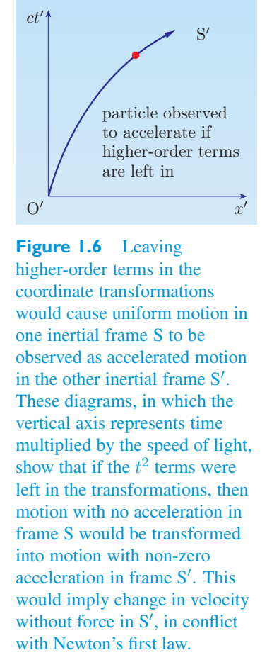
The transformations in Equations 1.18 and 1.19 can be further simplified by the requirement that the observers are using inertial frames of reference. Since Newton’s first law must hold in all inertial frames of reference, it is necessary that an object not accelerating in one set of coordinates is also not accelerating in the other set of coordinates. If the higher-order terms in and were not zero, then an object observed to have no acceleration in S (such as a spaceship with its thrusters off moving on the line, shown in the upper part of Figure 1.6) would be observed to accelerate in terms of \(x'\) and \(t'\) (i.e. \(x'_{3}\) = \(v'\) \(t'\), as indicated in the lower part of Figure 1.6). Observer O would report no force on the spaceship, while observer O would report some unknown force acting on it. In this way, the two observers would register different laws of physics, violating the first postulate of special relativity. The higher-order terms are therefore inconsistent with the required physics and must be removed, leaving only a linear transformation.方程 1.18 和 1.19 中的变换可以通过观察者使用惯性参考系的要求进一步简化。由于牛顿第一定律必须适用于所有惯性参考系,因此在一组坐标中不加速的物体在另一组坐标中也必须不加速。如果和中的高阶项不为零,则观察到 S 中没有加速度的物体(例如推进器关闭的宇宙飞船沿直线移动,如图 1.6 的上半部分所示)将观察到以 \(x'\) 和 \(t'\) 形式加速(即 \(x'_{3}\) = \(v'\) \(t'\),如图下半部分所示) 1.6)。观察者 O 会报告宇宙飞船上没有受到任何力,而观察者 O 会报告有一些未知的力作用在其上。这样,两个观察者就会记录到不同的物理定律,违反狭义相对论第一假设。因此,高阶项与所需的物理特性不一致,必须删除,只留下线性变换。
So we expect the special relativistic coordinate transformation between two frames in standard configuration to be represented by linear equations of the form因此,我们期望标准配置中两个框架之间的狭义相对论坐标变换可以由以下形式的线性方程表示
The remaining task is to determine the coefficients a 1, a 2, b 1 and b 2.剩下的任务是确定系数 a 1、a 2、b 1 和 b 2。
To do this, use is made of known relations between coordinates in both frames of reference. The first step is to use the fact that at any time t, the origin of \(S'\) (which is always at \(x'\) = 0 in \(S'\)) will be at x = V t in S. It follows from Equation 1.21 that为此,需要利用两个参考系中的坐标之间的已知关系。第一步是利用这样一个事实:在任何时间 t,\(S'\) 的原点(始终位于 \(S'\) 中的 \(x'\) = 0)将位于 S 中的 x = V t。从公式 1.21 可以得出:
from which we see that从中我们看到
Dividing Equation 1.21 by Equation 1.20, and using Equation将方程 1.21 除以方程 1.20,并使用方程
Now, as a second step we can use the fact that at any time \(t'\), the origin of frame S (which is always at x = 0 in S) will be at \(x'\) = − V \(t'\) in \(S'\). Substituting these values for x and \(x'\) into Equation 1.23 gives现在,作为第二步,我们可以使用以下事实:在任何时间 \(t'\),框架 S 的原点(始终位于 S 中的 x = 0)将位于 \(S'\) 中的 \(x'\) = − V \(t'\)。将 x 和 \(x'\) 的这些值代入公式 1.23 得出
from which it follows that由此可见
If we now substitute a 1 = b 1 into Equation 1.23 and divide the numerator and denominator on the right-hand side by t, then如果我们现在将 a 1 = b 1 代入方程 1.23,并将右侧的分子和分母除以 t,则
As a third step, the coefficient a 2 can be found using the principle of the constancy of the speed of light. A pulse of light emitted in the positive x -direction from (ct = 0, x = 0) has speed c = \(x'\)/\(t'\) and also c = x/t. Substituting these values into Equation 1.25 gives第三步,可以利用光速恒定原理求出系数a 2。从 (ct = 0, x = 0) 沿正 x 方向发射的光脉冲的速度为 c = \(x'\)/\(t'\) 并且 c = x/t。将这些值代入公式 1.25 得出
which can be rearranged to give可以重新排列以给出
Now that a 2, b 1 and b 2 are known in terms of a 1, the coordinate transformations between the two frames can be written as既然a 2、b 1 和b 2 都以a 1 的形式已知,那么两个坐标系之间的坐标变换可以写为
All that remains for the fourth step is to find an expression for a 1. To do this, we first write down the inverse transformations to Equations第四步剩下的就是找到 1 的表达式。为此,我们首先写下方程的逆变换
1.27 and 1.28, which1.27 和 1.28,其中
are found by exchanging primes and replacing V by − V. (We are implicitly assuming that a 1 depends only on some even power of通过交换素数并用 − V 替换 V 可以找到。(我们隐含地假设 1 仅取决于
Substituting Equations 1.29 and 1.30 into Equation 1.28 gives将方程 1.29 和 1.30 代入方程 1.28 得出
The second and third terms involving a 1 V \(t'\) cancel in this expression, leaving an expression in which the \(x'\) cancels on both sides:涉及 1 V \(t'\) 的第二项和第三项在此表达式中取消,留下 \(x'\) 在两侧取消的表达式:
By rearranging this equation and taking the positive square root, the coefficient a is determined to be通过重新排列该方程并取正平方根,系数 a 确定为
Thus a 1 is seen to be the Lorentz factor \(\gamma(V)\), which completes the derivation.因此,1 被视为洛伦兹因子 \(\gamma(V)\),从而完成了推导。
Some further arguments allow the Lorentz transformations to be extended to one time and three space dimensions. There can be no y and z contributions to the transformations for \(t'\) and \(x'\) since the y - and z -axes could be oriented in any of the perpendicular directions without affecting the events on the x -axis. Similarly, there can be no contributions to the transformations for \(y'\) and \(z'\) from any other coordinates, as space would become distorted in a non-symmetric manner.一些进一步的论点允许洛伦兹变换扩展到一维和三维空间。 \(t'\) 和 \(x'\) 的变换不会有 y 和 z 贡献,因为 y 轴和 z 轴可以沿任何垂直方向定向,而不影响 x 轴上的事件。类似地,任何其他坐标对 \(y'\) 和 \(z'\) 的变换都没有贡献,因为空间会以非对称方式扭曲。
1.2.4 Intervals and their transformation rules1.2.4 区间及其变换规则
Knowing how the coordinates of an event transform from one frame to another, it is relatively simple to determine how the coordinate intervals that separate pairs of events transform. As you will see in the next section, the rules for transforming intervals are often very useful.了解事件的坐标如何从一帧变换到另一帧,确定分隔事件对的坐标间隔如何变换就相对简单。正如您将在下一节中看到的,转换间隔的规则通常非常有用。
Intervals间隔
An interval between two events, measured along a specified axis in a given frame of reference, is the difference in the corresponding coordinates of the two events.在给定参考系中沿指定轴测量的两个事件之间的间隔是两个事件的相应坐标的差值。
To develop transformation rules for intervals, consider the Lorentz transformations for the coordinates of two events labelled 1 and 2:要制定间隔的变换规则,请考虑标记为 1 和 2 的两个事件的坐标的洛伦兹变换:
Subtracting the transformation equation for \(t'_{1}\) from that for \(t'_{2}\), and subtracting the transformation equation for \(x'_{1}\) from that for \(x'_{2}\), and so on, gives the following transformation rules for intervals:从 \(t'_{2}\) 的变换方程中减去 \(t'_{1}\) 的变换方程,从 \(x'_{2}\) 的变换方程中减去 \(x'_{1}\) 的变换方程,依此类推,给出以下区间变换规则:
where \(\Delta t = t\)− t, \(\Delta x = x\)− x, \(\Delta y = y\)− y and \(\Delta z = z\)− z denote the various time and space intervals between the events. The inverse transformations V: for intervals have the same form, with V replaced by −其中 \(\Delta t = t\)− t、\(\Delta x = x\)− x、\(\Delta y = y\)− y 和 \(\Delta z = z\)− z 表示事件之间的各种时间和空间间隔。区间的逆变换 V: 具有相同的形式,其中 V 替换为 -
The transformation rules for intervals are useful because they depend only on coordinate differences and not on the specific locations of events in time or space.间隔的变换规则很有用,因为它们仅取决于坐标差异,而不取决于事件在时间或空间中的具体位置。
1.3 Consequences of the Lorentz transformations1.3 洛伦兹变换的结果
In this section, some of the extraordinary consequences of the Lorentz transformations will be examined. In particular, we shall consider the findings of different observers regarding the rate at which a clock ticks, the length of a rod and the simultaneity of a pair of events. In each case, the trick for determining how the relevant property transforms between frames of reference is to carefully specify how intuitive concepts such as length or duration should be defined consistently in different frames of reference. This is most easily done by identifying each concept with an appropriate interval between two events: 1 and在本节中,将研究洛伦兹变换的一些非凡后果。特别是,我们将考虑不同观察者关于时钟走动的速度、杆的长度和一对事件的同时性的发现。在每种情况下,确定相关属性如何在参考系之间转换的技巧是仔细指定如何在不同参考系中一致地定义直观概念(例如长度或持续时间)。最容易做到这一点的方法是通过两个事件之间的适当间隔来识别每个概念:1 和
2. Once this has been achieved, we can determine which2. 一旦实现了这一点,我们就可以确定
intervals are known and then use the interval transformation rules (Equations 1.32–1.35 and 1.36–1.39) to find relationships between them. The rest of this section will give examples of this process.区间已知,然后使用区间变换规则(方程 1.32-1.35 和 1.36-1.39)来查找它们之间的关系。本节的其余部分将给出此过程的示例。
1.3.1 Time dilation1.3.1 时间膨胀
One of the most celebrated consequences of special relativity is the finding that ‘moving clocks run slow’. More precisely, any inertial observer must observe that the clocks used by another inertial observer, in uniform relative motion, will run slow. Since clocks are merely indicators of the passage of time, this is really the assertion that any inertial observer will find that time passes more slowly for any other inertial observer who is in relative motion. Thus, according to special relativity, if you and I are inertial observers, and we are in uniform relative motion, then I can perform measurements that will show that time is passing more slowly for you and, simultaneously, you can perform measurements that will show that time is passing more slowly for me. Both of us will be right because time is a relative quantity, not an absolute one. To show how this effect follows from the Lorentz transformations, it is essential to introduce clear, unambiguous definitions of the time intervals that are to be related.狭义相对论最著名的结论之一是发现“移动的时钟运行缓慢”。更准确地说,任何惯性观察者都必须观察到另一个惯性观察者使用的时钟在匀速相对运动中会走慢。由于时钟仅仅是时间流逝的指示器,这实际上是这样的断言:任何惯性观察者都会发现,对于任何其他相对运动的惯性观察者来说,时间过得更慢。因此,根据狭义相对论,如果你和我是惯性观察者,并且我们处于匀速相对运动,那么我可以进行测量,表明时间对你来说流逝得更慢,同时,你也可以进行测量来表明时间对我来说流逝得更慢。我们俩都是对的,因为时间是一个相对量,而不是绝对量。为了展示洛伦兹变换如何产生这种效应,有必要引入相关时间间隔的清晰、明确的定义。
Rather than deal with ticking clocks, our discussion here will refer to short-lived sub-nuclear particles of the sort routinely studied at CERN and other particle physics laboratories. For the purpose of the discussion, a short-lived particle is considered to be a point-like object that is created at some event, labelled 1, and subsequently decays at some other event, labelled 2. The time interval between these two events, as measured in any particular inertial frame, is the lifetime of the particle in that frame. This interval is analogous to the time between successive ticks of a clock.我们在这里讨论的不是滴答作响的时钟,而是欧洲核子研究中心和其他粒子物理实验室常规研究的那种短命亚核粒子。出于讨论的目的,短寿命粒子被认为是在某个事件中创建的点状物体,标记为 1,随后在某个其他事件中衰变,标记为 2。在任何特定惯性系中测量的这两个事件之间的时间间隔就是该系中粒子的寿命。该间隔类似于时钟连续滴答之间的时间。
We shall consider the lifetime of a particular particle as observed by two different inertial observers O and \(O'\). Observer O uses a frame S that is fixed in the laboratory, in which the particle travels with constant speed V in the positive x -direction. We shall call this the laboratory frame. Observer \(O'\) uses a frame S that moves with the particle. Such a frame is called the rest frame of the particle since the particle is always at rest in that frame. (You can think of the observer O as riding on the particle if you wish.)我们将考虑由两个不同的惯性观察者 O 和 \(O'\) 观察到的特定粒子的寿命。观察者 O 使用固定在实验室中的框架 S,其中粒子以恒定速度 V 沿正 x 方向行进。我们将其称为实验室框架。观察者 \(O'\) 使用随粒子移动的坐标系 S。这样的坐标系称为粒子的静止坐标系,因为粒子在该坐标系中始终处于静止状态。 (如果你愿意的话,你可以将观察者 O 想象成骑在粒子上。)
According to observer \(O'\), the birth and decay of the (stationary) particle happen at the same place, so if event 1 occurs at (\(t'\), \(x'\)), then event 2 occurs at (\(t'\), \(x'\)), and the lifetime of the particle will be \(\Delta t'\) = \(t'_{2}\) − \(t'_{1}\). In special relativity, the time between two events measured in a frame in which the events happen at the same position is called the proper time between the events and is usually denoted by the symbol \(\Delta \tau\). So, in this case, we can say that in frame \(S'\) the intervals of time and space that separate the two events are \(\Delta t'\) = \(\Delta \tau =\)\(t'\) − \(t'\) and \(\Delta x'\) = 0.根据观察者 \(O'\),(静止)粒子的诞生和衰变发生在同一个地方,因此如果事件 1 发生在(\(t'\),\(x'\)),那么事件 2 发生在(\(t'\),\(x'\)),粒子的寿命将为 \(\Delta t'\) = \(t'_{2}\) − \(t'_{1}\)。在狭义相对论中,在事件发生在同一位置的框架中测量的两个事件之间的时间称为事件之间的固有时间,通常用符号 \(\Delta \tau\) 表示。因此,在这种情况下,我们可以说,在帧 \(S'\) 中,分隔两个事件的时间和空间间隔为 \(\Delta t'\) = \(\Delta \tau =\)\(t'\) − \(t'\) 且 \(\Delta x'\) = 0。
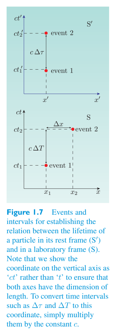
According to observer O in the laboratory frame S, event 1 occurs at (t 1, \(x^1\)) and event 2 at (\(t_{2}\), \(x_{2}\)), and the lifetime of the particle is \(\Delta t = t_{2}\)− t 1, which we shall call \(\Delta T\). Thus in frame S the intervals of time and space that separate the two events are \(\Delta t =\)\(\Delta T = t\)− t and \(\Delta x = x\)− x.根据实验室坐标系 S 中的观察者 O,事件 1 发生在 (t 1, \(x^1\)),事件 2 发生在 (\(t_{2}\), \(x_{2}\)),粒子的寿命为 \(\Delta t = t_{2}\)− t 1,我们将其称为 \(\Delta T\)。因此,在坐标系 S 中,分隔两个事件的时间和空间间隔为 \(\Delta t =\)\(\Delta T = t\)− t 和 \(\Delta x = x\)− x。
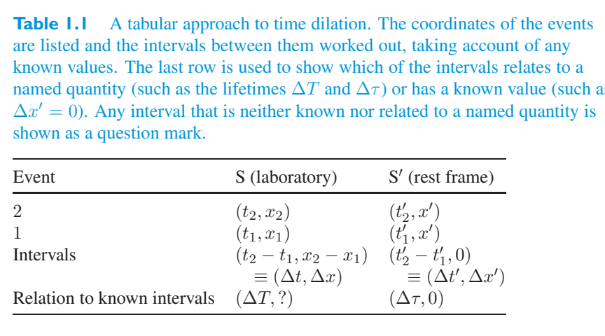
These events and intervals are represented in Figure 1.7, and everything we know about them is listed in Table 1.1. Such a table is helpful in establishing which of the interval transformations will be useful.这些事件和间隔如图 1.7 所示,表 1.1 列出了我们对它们的了解。这样的表有助于确定哪些区间变换有用。
Table 1.1 A tabular approach to time dilation. The coordinates of the events are listed and the intervals between them worked out, taking account of any known values. The last row is used to show which of the intervals relates to a named quantity (such as the lifetimes \(\Delta T\) and \(\Delta \tau\)) or has a known value (such as \(\Delta x'\) = 0). Any interval that is neither known nor related to a named quantity is shown as a question mark.表 1.1 时间膨胀的表格方法。列出事件的坐标并计算出事件之间的间隔,同时考虑到任何已知值。最后一行用于显示哪个间隔与命名量相关(例如寿命 \(\Delta T\) 和 \(\Delta \tau\))或具有已知值(例如 \(\Delta x'\) = 0)。任何既不已知也不与命名量相关的区间都显示为问号。
are listed and the intervals between them worked out, taking account of any known values. The last row is used to show which of the intervals relates to a named quantity (such as the lifetimes \(\Delta T\) and \(\Delta \tau\)) or has a known value (such as \(\Delta x'\) = 0). Any interval that is neither known nor related to a named quantity is shown as a question mark.列出并计算出它们之间的间隔,同时考虑到任何已知值。最后一行用于显示哪个间隔与命名量相关(例如寿命 \(\Delta T\) 和 \(\Delta \tau\))或具有已知值(例如 \(\Delta x'\) = 0)。任何既不已知也不与命名量相关的区间都显示为问号。
Event S (laboratory) \(S'\) (rest frame)事件S(实验室)\(S'\)(休息架)
Intervals间隔
Relation to known intervals (\(\Delta T\),?)与已知间隔的关系(\(\Delta T\),?)
Each of the interval transformation rules that were introduced in the previous section involves three intervals. Only Equation 1.36 involves the three known intervals. Substituting the known intervals into that equation gives上一节中介绍的每个区间变换规则都涉及三个区间。只有方程 1.36 涉及三个已知区间。将已知区间代入该方程可得出
\(\Delta T =\)\(\gamma(V)\)(\(\Delta \tau + 0\)). Therefore the particle lifetimes measured in S and \(S'\) are related by\(\Delta T =\)\(\gamma(V)\)(\(\Delta\tau + 0\))。因此,以 S 和 \(S'\) 测量的颗粒寿命与下式相关:
Since \(\gamma(V)\) > 1, this result tells us that the particle is observed to live longer in the laboratory frame than it does in its own rest frame. This is an example of the effect known as time dilation. A process that occupies a (proper) time \(\Delta \tau\) in its own rest frame has a longer duration \(\Delta T\) when observed from some other frame that moves relative to the rest frame. If the process is the ticking of a clock, then a consequence is that moving clocks will be observed to run slow.由于 \(\gamma(V)\) > 1,该结果告诉我们,观察到粒子在实验室框架中的寿命比在其自身静止框架中的寿命更长。这是时间膨胀效应的一个例子。当从相对于静止坐标系移动的某个其他坐标系观察时,在其自身静止坐标系中占据(适当)时间 \(\Delta \tau\) 的过程具有较长的持续时间 \(\Delta T\)。如果这个过程是一个时钟的滴答声,那么结果就是移动的时钟会被观察到运行缓慢。
The time dilation effect has been demonstrated experimentally many times. It provides one of the most common pieces of evidence supporting Einstein’s theory of special relativity. If it did not exist, many experiments involving short-lived particles, such as muons, would be impossible, whereas they are actually quite routine.时间膨胀效应已被多次实验证明。它提供了支持爱因斯坦狭义相对论的最常见的证据之一。如果它不存在,许多涉及短寿命粒子(例如\(\mu\)子)的实验将是不可能的,而它们实际上是相当常规的。
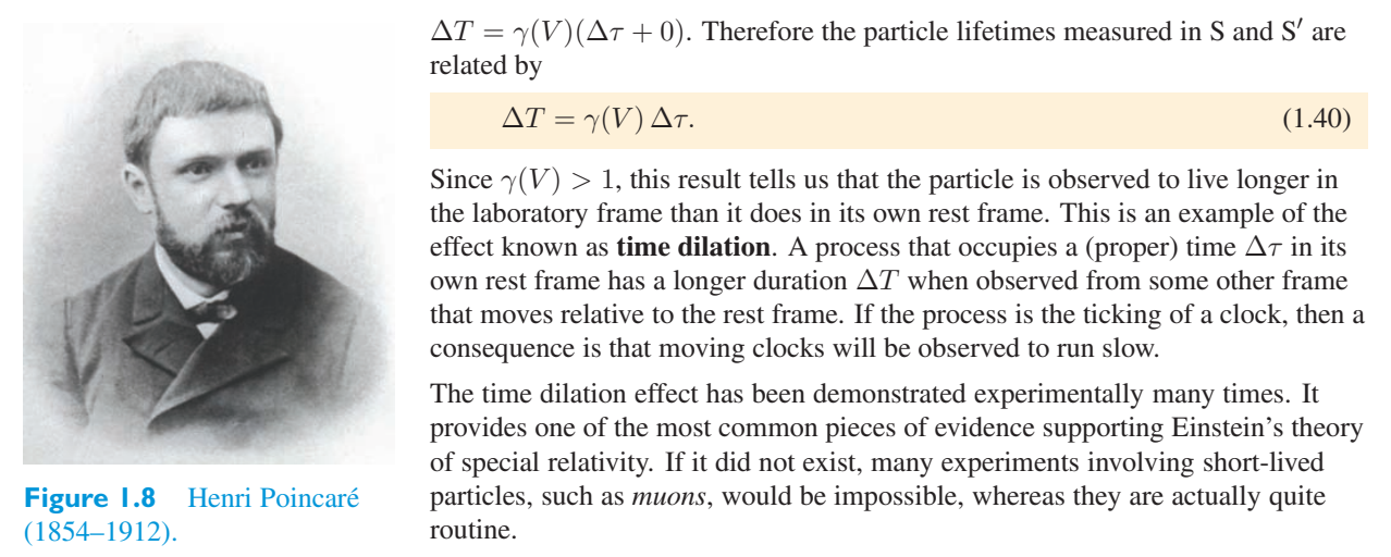
It is interesting to note that the French mathematician Henri Poincaré (Figure 1.8) proposed an effect similar to time dilation shortly before Einstein formulated special relativity.有趣的是,法国数学家亨利·庞加莱(Henri Poincaré)(图 1.8)在爱因斯坦提出狭义相对论之前不久就提出了类似于时间膨胀的效应。
Exercise 1.4 A particular muon lives for \(\Delta \tau = 2\).2练习 1.4 一个特定的 \(\mu\) 子存在于 \(\Delta \tau = 2\).2 中
\(\mu\) s in its own rest frame. If that muon is travelling with speed V = 3 c/5 relative to an observer on Earth, what is its lifetime as measured by that observer?\(\mu\) 位于其自己的休息框架中。如果该 \(\mu\) 子相对于地球上的观察者以 V = 3 c/5 的速度行进,那么该观察者测得的它的寿命是多少?
1.3.2 Length contraction1.3.2 长度收缩
There is another curious relativistic effect that relates to the length of an object observed from different frames of reference. For the sake of simplicity, the object that we shall consider is a rod, and we shall start our discussion with a definition of the rod’s length that applies whether or not the rod is moving.还有另一种奇怪的相对论效应,它与从不同参考系观察到的物体的长度有关。为了简单起见,我们要考虑的对象是一根杆,我们将从杆长度的定义开始讨论,无论杆是否移动,该定义都适用。
In any inertial frame of reference, the length of a rod is the distance between its \(x^1\) " 1 end-points at a single time as measured in that frame.在任何惯性参考系中,杆的长度是在该参考系中测量的单个时间点之间的 \(x^1\) " 1 端点之间的距离。
Thus, in an inertial frame S in which the rod is oriented along the x -axis and moves along that axis with constant speed V, the length L of the rod can be related to two events, 1 and 2, that happen at the ends of the rod at the same time t. If event 1 is at (t, \(x^1\)) and event 2 is at (t, \(x_{2}\)), then the length of the rod, as measured in S at time t, is given by L = \(\Delta x = x_{2}\)− x因此,在惯性系 S 中,杆沿 x 轴定向并以恒定速度 V 沿该轴移动,杆的长度 L 可以与在同一时间 t 发生在杆两端的两个事件 1 和 2 相关。如果事件 1 发生在 (t, \(x^1\)),事件 2 发生在 (t, \(x_{2}\)),则在时间 t 时在 S 中测量的杆长度由下式给出: L = \(\Delta x = x_{2}\)− x
1.1.
Now consider these same two events as observed in an inertial frame S in which the rod is oriented along the \(x'\)-axis but is always at rest. In this case we still know that event 1 and event 2 occur at the end-points of the rod, but we have no reason to suppose that they will occur at the same time, so we shall describe them by the coordinates (\(t'\), \(x'\)) and (\(t'\), \(x'\)). Although these events may not be simultaneous, we know that in frame \(S'\) the rod is not moving, so its end-points are always at \(x'_{1}\) and \(x'_{2}\). Consequently, we can say that the length of the rod in its own rest frame — a quantity sometimes referred to as the proper length of the rod and denoted L — is given by L = \(\Delta x'\) = \(x'\) − \(x'\).现在考虑在惯性系 S 中观察到的这两个相同的事件,其中杆沿着 \(x'\) 轴定向,但始终处于静止状态。在这种情况下,我们仍然知道事件 1 和事件 2 发生在杆的端点,但我们没有理由假设它们会同时发生,因此我们将通过坐标 (\(t'\), \(x'\)) 和 (\(t'\), \(x'\)) 来描述它们。尽管这些事件可能不是同时发生的,但我们知道在 \(S'\) 坐标系中,杆没有移动,因此其端点始终位于 \(x'_{1}\) 和 \(x'_{2}\)。因此,我们可以说,杆在其自身静止框架中的长度(有时称为杆的适当长度并表示为 L)由下式给出:L = \(\Delta x'\) = \(x'\) – \(x'\)。
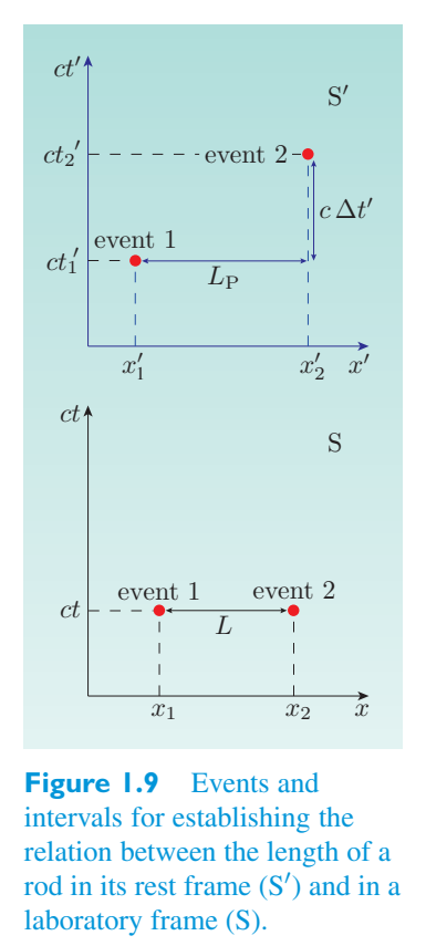
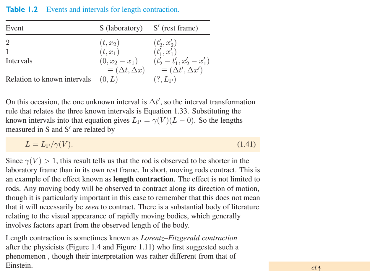
These events and intervals are represented in Figure 1.9, and everything we know about them is listed in Table 1.2.这些事件和间隔如图 1.9 所示,表 1.2 列出了我们对它们的了解。
Table 1.2 Events and intervals for length contraction.表 1.2 长度收缩的事件和间隔。
Event S (laboratory) \(S'\) (rest frame)事件S(实验室)\(S'\)(休息架)
Intervals间隔
Relation to known intervals (0, L)与已知区间 (0, L) 的关系
On this occasion, the one unknown interval is \(\Delta t'\), so the interval transformation rule that relates the three known intervals is Equation 1.33. Substituting the known intervals into that equation gives L P = \(\gamma(V)\)(L − 0). So the lengths measured in S and \(S'\) are related by此时,一个未知区间为\(\Delta t'\),因此将三个已知区间关联起来的区间变换规则为公式1.33。将已知区间代入该方程可得出 L P = \(\gamma(V)\)(L − 0)。因此,以 S 和 \(S'\) 测量的长度之间的关系为
Since \(\gamma(V)\) > 1, this result tells us that the rod is observed to be shorter in the laboratory frame than in its own rest frame. In short, moving rods contract. This is an example of the effect known as length contraction. The effect is not limited to rods. Any moving body will be observed to contract along its direction of motion, though it is particularly important in this case to remember that this does not mean that it will necessarily be seen to contract. There is a substantial body of literature relating to the visual appearance of rapidly moving bodies, which generally involves factors apart from the observed length of the body.由于 \(\gamma(V)\) > 1,该结果告诉我们,观察到杆在实验室框架中比在其自身的静止框架中更短。简而言之,移动的杆收缩。这是长度收缩效应的一个例子。效果不限于棒。任何移动的物体都会被观察到沿着其运动方向收缩,尽管在这种情况下特别重要的是要记住,这并不意味着它一定会被看到收缩。有大量关于快速移动物体的视觉外观的文献,这些文献通常涉及除观察到的物体长度之外的因素。
Length contraction is sometimes known as Lorentz–Fitzgerald contraction after the physicists (Figure 1.4 and Figure 1.11) who first suggested such a phenomenon, though their interpretation was rather different from that of Einstein.长度收缩有时被称为洛伦兹-菲茨杰拉德收缩,这是由首先提出这种现象的物理学家(图 1.4 和图 1.11)命名的,尽管他们的解释与爱因斯坦的解释截然不同。
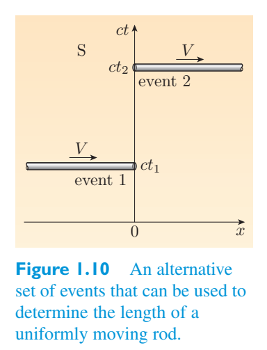
Exercise 1.5 There is an alternative way of defining length in frame S based练习 1.5 有一种基于 S 帧定义长度的替代方法
on two events, 1 and 2, that happen at different times in that frame. Suppose that event 1 occurs at x = 0 as the front end of the rod passes that point, and event 2 also occurs at x = 0 but at the later time when the rear end passes. Thus event 1 is at (t 1, 0) and event 2 is at (\(t_{2}\), 0). Since the rod moves with uniform speed V in frame S, we can define the length of the rod, as measured in S, by the relation L = V (\(t_{2}\) − t 1). Use this alternative definition of length in frame S to establish that the length of a moving rod is less than its proper length. (The events are represented in Figure 1.10.)两个事件(1 和 2)在该帧中的不同时间发生。假设事件 1 发生在杆前端经过该点时的 x = 0 处,事件 2 也发生在 x = 0 处,但发生在杆后端经过该点的较晚时间。因此,事件 1 位于 (t 1, 0),事件 2 位于 (\(t_{2}\), 0)。由于杆在坐标系 S 中以匀速 V 移动,因此我们可以通过关系式 L = V (\(t_{2}\) − t 1) 来定义在 S 中测量的杆的长度。使用 S 系中长度的替代定义来确定移动杆的长度小于其正确长度。 (这些事件如图 1.10 所示。)
1.3.3 The relativity of simultaneity1.3.3 同时性的相对性
It was noted in the discussion of length contraction that two events that occur at the same time in one frame do not necessarily occur at the same time in another frame. Indeed, looking again at Figure 1.9 and Table 1.2 but now calling on the interval transformation rule of Equation 1.32, it is clear that if the events 1 and 2 are observed to occur at the same time in frame S (so \(\Delta t = 0\)) but are separated by a distance L along the x -axis, then in frame \(S'\) they will be separated by the time在长度收缩的讨论中注意到,在一帧中同时发生的两个事件不一定在另一帧中同时发生。事实上,再次查看图 1.9 和表 1.2,但现在调用方程 1.32 的区间变换规则,很明显,如果观察到事件 1 和 2 在帧 S 中同时发生(因此 \(\Delta t = 0\)),但沿 x 轴相隔距离 L,则在帧 \(S'\) 中它们将被时间间隔
Two events that occur at the same time in some frame are said to be simultaneous in that frame. The above result shows that the condition of being simultaneous is a relative one not an absolute one; two events that are simultaneous in one frame are not necessarily simultaneous in every other frame. This consequence of the Lorentz transformations is referred to as the relativity of simultaneity.在某个帧中同时发生的两个事件被称为在该帧中同时发生。上述结果表明,同时的条件是相对的,而不是绝对的;一帧中同时发生的两个事件不一定在其他帧中同时发生。洛伦兹变换的这一结果被称为同时性相对性。
1.3.4 The Doppler effect1.3.4 多普勒效应
A physical phenomenon that was well known long before the advent of special relativity is the Doppler effect. This accounts for the difference between the emitted and received frequencies (or wavelengths) of radiation arising from the relative motion of the emitter and the receiver. You will have heard an example of the Doppler effect if you have listened to the siren of a passing ambulance: the frequency of the siren is higher when the ambulance is approaching (i.e. travelling towards the receiver) than when it is receding (i.e. travelling away from the receiver).在狭义相对论出现之前很久就众所周知的物理现象是多普勒效应。这解释了由于发射器和接收器的相对运动而产生的辐射的发射和接收频率(或波长)之间的差异。如果您听过经过的救护车的警报声,您就会听到多普勒效应的一个例子:当救护车接近(即朝接收器行驶)时警报器的频率比救护车后退(即远离接收器行驶)时的频率更高。
Astronomers routinely use the Doppler effect to determine the speed of approach or recession of distant stars. They do this by measuring the received wavelengths of narrow lines in the star’s spectrum, and comparing their results with the proper wavelengths of those lines that are well known from laboratory measurements and represent the wavelengths that would have been emitted in the star’s rest frame.天文学家通常使用多普勒效应来确定遥远恒星接近或后退的速度。他们通过测量恒星光谱中窄线的接收波长,并将其结果与实验室测量中众所周知的那些线的正确波长进行比较,这些线代表了恒星静止框架中发射的波长。
Despite the long history of the Doppler effect, one of the consequences of special relativity was the recognition that the formula that had traditionally been used to describe it was wrong. We shall now obtain the correct formula.尽管多普勒效应有着悠久的历史,但狭义相对论的后果之一是人们认识到传统上用来描述它的公式是错误的。现在我们将获得正确的公式。
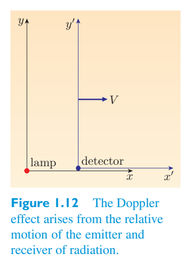
Consider a lamp at rest at the origin of an inertial frame S emitting electromagnetic waves of proper frequency f em as measured in S. Now suppose that the lamp is observed from another inertial frame \(S'\) that is in standard configuration with S, moving away at constant speed V (see Figure 1.12). A detector fixed at the origin of \(S'\) will show that the radiation from the receding lamp is received with frequency f rec as measured in \(S'\). Our aim is to find the relationship between f rec and f em.考虑一盏静止在惯性系 S 原点的灯,发射在 S 中测量的适当频率 f em 的电磁波。现在假设从另一个与 S 处于标准配置的惯性系 \(S'\) 观察该灯,以恒定速度 V 移动(见图 1.12)。固定在 \(S'\) 原点的检测器将显示来自后退灯的辐射以 \(S'\) 测量的频率 f rec 被接收。我们的目标是找到 f rec 和 fem 之间的关系。
The emitted waves have regularly positioned nodes that are separated by a proper wavelength \(\lambda\) em = \(f_{\rm em}\)/c as measured in S. In that frame the time interval between the emission of one node and the next, \(\Delta t\), represents the proper period of the wave, T em, so we can write \(\Delta t = T em\)= 1/\(f_{\rm em}\).发射的波具有规则定位的节点,这些节点以适当的波长 \(\lambda\) em = \(f_{\rm em}\)/c 分隔开,如在 S 中测量的。在该帧中,一个节点与下一个节点发射之间的时间间隔 \(\Delta t\) 代表波的适当周期 T em,因此我们可以写成 \(\Delta t = T em\)= 1/\(f_{\rm em}\)。
Due to the phenomenon of time dilation, an observer in frame \(S'\) will find that the time separating the emission of successive nodes is \(\Delta t' = \gamma(V)\Delta t\). However, this is not the time that separates the arrival of those nodes at the detector because the detector is moving away from the emitter at a constant rate. In fact, during the interval \(\Delta t'\) the detector will increase its distance from the emitter by \(V\Delta t'\) as measured in \(S'\), and this will cause the reception of the two nodes to be separated by a total time \(\Delta t' + V\Delta t'/c\) as measured in \(S'\). This represents the received period of the wave and is therefore the reciprocal of the received frequency, so we can write由于时间膨胀现象,在 \(S'\) 坐标系中的观察者会发现连续节点发射的时间间隔为 \(\Delta t'\) = \(\gamma(V)\) \(\Delta t\)。然而,这并不是这些节点到达检测器的时间间隔,因为检测器以恒定的速率远离发射器。事实上,在时间间隔 \(\Delta t'\) 内,检测器与发射器的距离将增加 V \(\Delta t'\)(以 \(S'\) 为单位测量),这将导致两个节点的接收间隔总时间 \(\Delta t'\) + V \(\Delta t'\)/c(以 \(S'\) 为单位测量)。这代表了波的接收周期,因此是接收频率的倒数,所以我们可以写
We can now identify - \(\Delta t\) with the reciprocal of the emitted frequency and use the identity \(\gamma(V)\) = 1/(1 − V/c)(1 + V/c) to write现在我们可以用发射频率的倒数来表示 - \(\Delta t\),并使用恒等式 \(\gamma(V)\) = 1/(1 − V/c)(1 + V/c) 来写出
which can be rearranged to give可以重新排列以给出
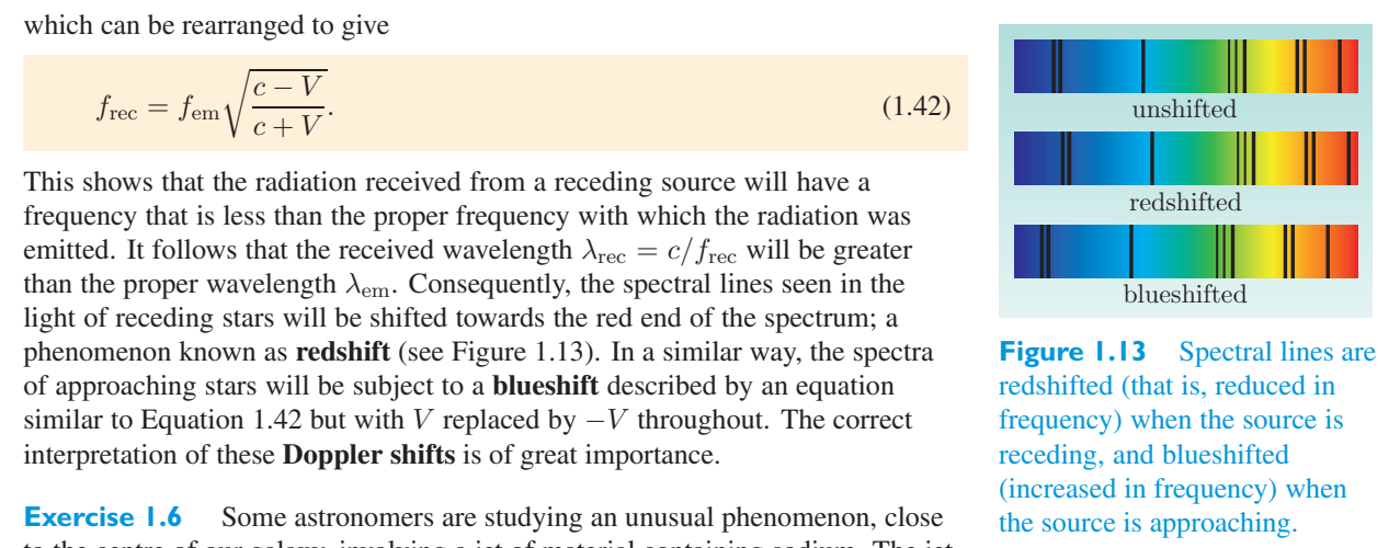
This shows that the radiation received from a receding source will have a frequency that is less than the proper frequency with which the radiation was emitted. It follows that the received wavelength \(\lambda\) rec = c/\(f_{\rm rec}\) will be greater than the proper wavelength \(\lambda\) em. Consequently, the spectral lines seen in the light of receding stars will be shifted towards the red end of the spectrum; a phenomenon known as redshift (see Figure 1.13). In a similar way, the spectra of approaching stars will be subject to a blueshift described by an equation similar to Equation 1.42 but with V replaced by − V throughout. The correct interpretation of these Doppler shifts is of great importance.这表明从后退源接收到的辐射的频率将小于发射辐射的适当频率。由此可见,接收波长 \(\lambda\) rec = c/\(f_{\rm rec}\) 将大于适当波长 \(\lambda\) em。因此,在后退恒星的光线下看到的光谱线将向光谱的红端移动;这种现象称为红移(见图 1.13)。以类似的方式,接近恒星的光谱将受到蓝移的影响,该蓝移由类似于方程 1.42 的方程描述,但 V 始终替换为 - V。对这些多普勒频移的正确解释非常重要。
Exercise 1.6 Some astronomers are studying an unusual phenomenon, close练习 1.6 一些天文学家正在研究一种不寻常的现象,接近
to the centre of our galaxy, involving a jet of material containing sodium. The jet is moving almost directly along the line between the Earth and the galactic centre. In a laboratory, a stationary sample of sodium vapour absorbs light of wavelength \(\lambda\) = \(5850\times10^{-10}\) m. Spectroscopic studies show that the wavelength of the sodium absorption line in the jet’s spectrum is \(\lambda'\) = \(4483\times10^{-10}\) m. Is the jet approaching or receding? What is the speed of the jet relative to Earth? (Note that the main challenge in this question is the mathematical one of using Equation 1.42 to obtain an expression for V in terms of \(\lambda\)/\(\lambda'\).)到我们银河系的中心,涉及到一股含有钠的物质射流。这架喷射机几乎直接沿着地球和银河中心之间的线移动。在实验室中,钠蒸气的固定样品吸收波长为 \(\lambda\) = \(5850\times10^{-10}\) m 的光。光谱研究表明,射流光谱中钠吸收线的波长为 \(\lambda'\) = \(4483\times10^{-10}\) m。喷气式飞机正在接近还是正在后退?喷气机相对于地球的速度是多少? (请注意,此问题的主要挑战是使用公式 1.42 获得以 \(\lambda\)/\(\lambda'\) 表示的 V 表达式。)
1.3.5 The velocity transformation1.3.5 速度变换
Suppose that an object is observed to be moving with velocity v = (\(v_{x}\), \(v_{y}\), \(v_{z}\)) in an inertial frame S. What will its velocity be in a frame \(S'\) that is in standard configuration with S, travelling with uniform speed V in the positive x -direction? The Galilean transformation would lead us to expect \(v'\) = (\(v_{x}\) − V, \(v_{y}\), \(v_{z}\)), but we know that is not consistent with the observed behaviour of light. Once again we shall use the interval transformation rules that follow directly from the Lorentz transformations to find the velocity transformation rule according to special relativity.假设观察到一个物体在惯性系 S 中以速度 v = (\(v_{x}\), \(v_{y}\), \(v_{z}\)) 移动。在与 S 处于标准配置的系 \(S'\) 中,该物体以匀速 V 沿正 x 方向行进,其速度是多少?伽利略变换会让我们期望 \(v'\) = (\(v_{x}\) − V, \(v_{y}\), \(v_{z}\)),但我们知道这与观察到的光行为不一致。我们将再次使用直接源自洛伦兹变换的区间变换规则来根据狭义相对论找到速度变换规则。
We know from Equations 1.32 and 1.33 that the time and space intervals between two events 1 and 2 that occur on the x -axis in frame S, transform according to从方程 1.32 和 1.33 可知,S 帧中 x 轴上发生的两个事件 1 和 2 之间的时间和空间间隔,根据以下变换:
Dividing the second of these equations by the first gives将这些方程中的第二个方程除以第一个方程得到
Dividing the upper and lower expressions on the right-hand side of this equation by \(\Delta t\), and cancelling the Lorentz factors, gives将该方程右侧的上式和下式表达式除以 \(\Delta t\),并取消洛伦兹因子,得到
Now, if we suppose that the two events that we are considering are very close together — indeed, if we consider the limit as \(\Delta t\) and \(\Delta x\) go to zero — then the quantities \(\Delta x\)/\(\Delta t\) and \(\Delta x'\)/\(\Delta t'\) will become the instantaneous velocity components \(v_{x}\) and v \(x'\) of a moving object that passes through the events 1 and 2. Extending these arguments to three dimensions by considering events that are not confined to the x -axis leads to the following velocity transformation rules:现在,如果我们假设我们正在考虑的两个事件非常接近 - 事实上,如果我们将极限视为 \(\Delta t\) 和 \(\Delta x\) 趋近于零 - 那么量 \(\Delta x\)/\(\Delta t\) 和 \(\Delta x'\)/\(\Delta t'\) 将成为穿过事件 1 和 2 的移动物体的瞬时速度分量 \(v_{x}\) 和 v \(x'\)。通过考虑不限于 x 轴的事件将这些参数扩展到三个维度,从而得出以下速度变换规则:
These equations may look rather odd at first sight but they make good sense in the context of special relativity. When \(v_{x}\) and V are small compared to the speed of light c, the term \(v_{x}\) V/\(c^2\) is very small and the denominator is approximately 1. In \(x'\) = \(v_{x}\) − V, is recovered such cases, the Galilean velocity transformation rule, v as a low-speed approximation to the special relativistic result. At high speeds the situation is even more interesting, as the following question will show.这些方程乍一看可能相当奇怪,但在狭义相对论的背景下它们很有意义。当 \(v_{x}\) 和 V 与光速 c 相比较小时,\(v_{x}\) V/\(c^2\) 项非常小,分母约为 1。在 \(x'\) = \(v_{x}\) − V 中,恢复了这种情况下的伽利略速度变换规则,v 作为狭义相对论结果的低速近似。在高速情况下,情况甚至更加有趣,正如下面的问题所示。
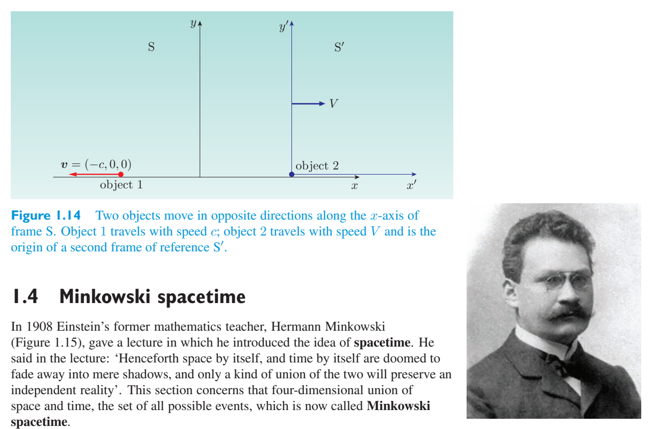
- ● An observer has established that two objects are receding● 观察者已确定两个物体正在后退
in opposite directions. Object 1 has speed c, and object 2 has speed V. Using the velocity transformation, compute the velocity with which object 1 recedes as measured by an observer travelling on object 2.在相反的方向。对象 1 的速度为 c,对象 2 的速度为 V。使用速度变换,计算在对象 2 上行进的观察者测量到的对象 1 后退的速度。
❍ Let the line along which the objects are travelling be the x -axis of the original observer’s frame, S. We can then suppose that a frame of reference \(S'\) that has its origin on object 2 is in standard configuration with frame S, and apply the velocity transformation to the velocity components of object 1 with v = (− c, 0, 0) (see Figure 1.14). The velocity transformation predicts that as 0, 0), where observed in \(S'\), the velocity of object 2 is \(v'\) = (\(v'\),❍ 设物体沿其移动的线为原始观察者坐标系 S 的 x 轴。然后,我们可以假设原点位于物体 2 上的参考系 \(S'\) 与坐标系 S 处于标准配置,并将速度变换应用于物体 1 的速度分量,其中 v = (− c, 0, 0)(见图 1.14)。速度变换预测为 0, 0),在 \(S'\) 中观察到,物体 2 的速度为 \(v'\) = (\(v'\),
So, as observed from object 2, object 1 is travelling in the − \(x'\)-direction at the speed of light, c. This was inevitable, since the second postulate of special relativity (which was used in the derivation of the Lorentz transformations) tells us that all observers agree about the speed of light. It is nonetheless pleasing to see how the velocity transformation delivers the required result in this case. It is worth noting that this result does not depend on the value of V.因此,从物体 2 观察到,物体 1 正在以光速 c 沿 - \(x'\) 方向行进。这是不可避免的,因为狭义相对论的第二假设(用于洛伦兹变换的推导)告诉我们所有观察者都同意光速。尽管如此,在这种情况下,看到速度变换如何提供所需的结果还是令人高兴的。值得注意的是,这个结果并不依赖于V的值。
Exercise 1.7 According to an observer on a spacestation,练习 1.7 根据空间站观察员的说法,
two spacecraft are moving away, travelling in the same direction at different speeds. The nearer spacecraft is moving at speed c/2, the further at speed 3 c/4. What is the speed of one of the spacecraft as observed from the other?两艘航天器正在远离,以不同的速度朝同一方向行驶。较近的航天器以 c/2 的速度移动,较远的航天器以 3 c/4 的速度移动。从其中一艘航天器观察到另一艘航天器的速度是多少?
1.4 Minkowski spacetime1.4 闵可夫斯基时空
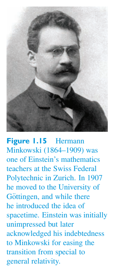
In 1908 Einstein’s former mathematics teacher, Hermann Minkowski (Figure 1.15), gave a lecture in which he introduced the idea of spacetime. He said in the lecture: ‘Henceforth space by itself, and time by itself are doomed to fade away into mere shadows, and only a kind of union of the two will preserve an independent reality’. This section concerns that four-dimensional union of space and time, the set of all possible events, which is now called Minkowski spacetime.1908 年,爱因斯坦的前数学老师赫尔曼·闵可夫斯基(Hermann 闵可夫斯基,图 1.15)在一次演讲中介绍了时空的概念。他在演讲中说:“从此以后,空间本身和时间本身都注定会消失在纯粹的阴影中,只有两者的某种结合才能保留一个独立的现实”。本节涉及空间和时间的四维联合,即所有可能事件的集合,现在称为闵可夫斯基时空。
1.4.1 Spacetime diagrams, lightcones and causality1.4.1 时空图、光锥和因果关系
We have already seen how the Lorentz transformations lead to some very counter-intuitive consequences. This subsection introduces a graphical tool known as a spacetime diagram or a Minkowski diagram that will help you to visualize events in Minkowski spacetime and thereby develop a better intuitive understanding of relativistic effects. The spacetime diagram for a frame of reference S is usually presented as a plot of ct against x, and each point on the diagram represents a possible event as observed in frame S. The y - and z -coordinates are usually ignored.我们已经看到洛伦兹变换如何导致一些非常违反直觉的后果。本小节介绍一种称为时空图或闵可夫斯基图的图形工具,它将帮助您可视化闵可夫斯基时空中的事件,从而更好地直观地理解相对论效应。参考系 S 的时空图通常表示为 ct 相对于 x 的图,图中的每个点代表在 S 系中观察到的一个可能事件。y 和 z 坐标通常被忽略。
Given two inertial frames, S and \(S'\), in standard configuration, it is instructive to plot the \(ct'\)- and \(x'\)-axes of frame \(S'\) on the spacetime diagram for frame S. The \(x'\)-axis of frame \(S'\) is defined by the set of events for which \(ct'\) = 0, and the \(ct'\)-axis is defined by the set of events for which \(x'\) = 0. The coordinates of these events in S are related to their coordinates in \(S'\) by the following Lorentz transformations. (Note that the time transformation of Equation 1.5 has been multiplied by c so that each coordinate can be measured in units of length.)给定两个惯性系 S 和 \(S'\),在标准配置中,在系 S 的时空图上绘制系统 \(S'\) 的 \(ct'\) 轴和 \(x'\) 轴是有益的。系统 \(x'\) 的 \(x'\) 轴由 \(ct'\) = 0 的事件集定义,并且\(ct'\) 轴由 \(x'\) = 0 的事件集定义。这些事件在 S 中的坐标通过以下洛伦兹变换与它们在 \(S'\) 中的坐标相关。 (请注意,公式 1.5 的时间变换已乘以 c,以便可以以长度单位测量每个坐标。)
Setting \(ct'\) = 0 in the first of these equations gives 0 = \(\gamma(V)\)(ct − V x/c). This shows that in the spacetime diagram for frame S, the \(ct'\)-axis of frame \(S'\) is represented by the line ct = (V/c) x, a straight line through the origin with gradient V/c. Similarly, setting \(x'\) = 0 in the second transformation equation gives 0 = \(\gamma(V)\)(x − V t), showing that the \(x'\)-axis of frame \(S'\) is represented by the line ct = (c/V) x, a straight line through the origin with gradient c/V in the spacetime diagram of S. These lines are shown in Figure在第一个方程中设置 \(ct'\) = 0 得出 0 = \(\gamma(V)\)(ct − V x/c)。这表明,在坐标系 S 的时空图中,坐标系 \(S'\) 的 \(ct'\) 轴由线 ct = (V/c) x 表示,这是一条通过原点且梯度为 V/c 的直线。类似地,在第二个变换方程中设置 \(x'\) = 0 得到 0 = \(\gamma(V)\)(x − V t),表明框架 \(S'\) 的 \(x'\) 轴由线 ct = (c/V) x 表示,这条直线穿过原点,在 S 的时空图中具有梯度 c/V。这些线如图所示
1.16.1.16。
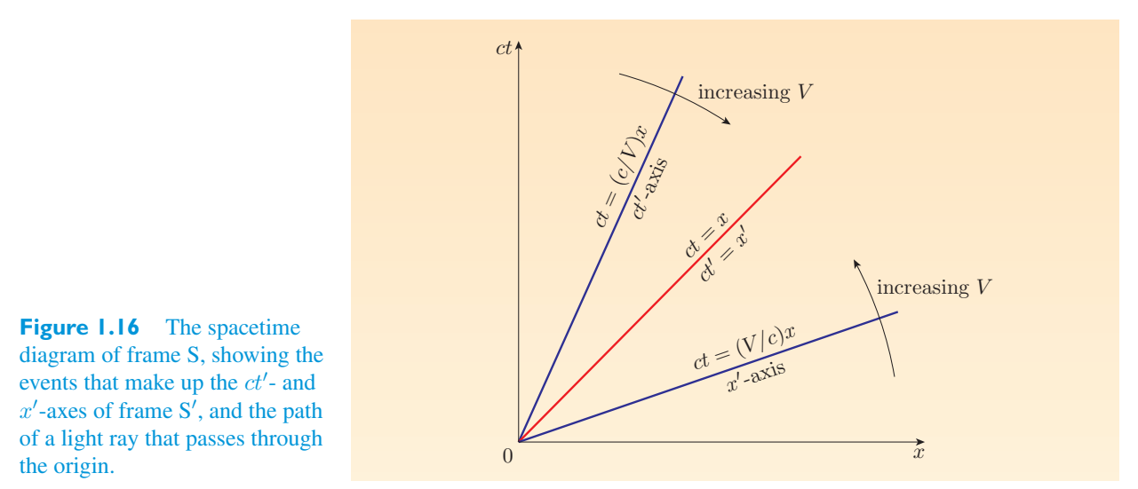
There is another feature of interest in the diagram. The straight line through the origin of gradient 1 links all the events where x = ct and thus shows the path of a light ray that passes through x = 0 at time t =该图中还有另一个有趣的特征。通过梯度 1 原点的直线联络了 x = ct 处的所有事件,因此显示了在时间 t = 时穿过 x = 0 的光线的路径
0. Using the inverse0. 使用逆
Lorentz transformations shows that this line also passes through all the events where \(\gamma(V)\)(\(x'\) + V \(t'\)) = \(\gamma(V)\)(\(ct'\) + V \(x'\)/c), that is (after some cancelling and rearranging), where \(x'\) = \(ct'\). So the line of gradient 1 passing through the origin also represents the path of a light ray that passes through the origin of frame \(S'\) at \(t'\) = 0. In fact, any line with gradient 1 on a spacetime diagram must always represent the possible path of a light ray, and thanks to the second postulate of special relativity, we can be sure that all observers will agree about that.洛伦兹变换表明,这条线还经过 \(\gamma(V)\)(\(x'\) + V \(t'\)) = \(\gamma(V)\)(\(ct'\) + V \(x'\)/c) 的所有事件,即(经过一些取消和重新排列后),其中 \(x'\) = \(ct'\)。因此,穿过原点的梯度 1 的线也代表光线在 \(t'\) = 0 处穿过坐标系 \(S'\) 的原点的路径。事实上,时空图上任何梯度为 1 的线都必须始终代表光线的可能路径,并且由于狭义相对论的第二假设,我们可以确信所有观察者都会同意这一点。
As the relative speed V of the frames S and \(S'\) increases, the lines representing the \(x'\)- and \(ct'\)-axes of \(S'\) close in on the line of gradient 1 from either side, rather like the closing of a clapper board. This behaviour reflects the fact that Lorentz transformations will generally alter the coordinates of events but will not change the behaviour of light on which all observers must agree.随着框架 S 和 \(S'\) 的相对速度 V 的增加,表示 \(S'\) 的 \(x'\) 轴和 \(ct'\) 轴的线从两侧向梯度 1 线靠拢,就像关闭拍板一样。这种行为反映了这样一个事实:洛伦兹变换通常会改变事件的坐标,但不会改变所有观察者必须同意的光的行为。
In the somewhat unusual case when we include a second spatial axis (the y -axis, say) in the spacetime diagram, the original line of gradient 1 is seen to be part of a cone, as indicated in Figure 1.17. This cone, which connects the event at the origin to all those events, past and future, that might be linked to it by a signal travelling at the speed of light, is an example of a lightcone. A horizontal slice (at ct = constant) through the (pseudo) three-dimensional diagram at any particular time shows a circle, but in a fully four-dimensional diagram with all three spatial axes included, such a fixed-time slice would be a sphere, and would represent a spherical shell of light surrounding the origin. At times earlier than t = 0, the shell would represent incoming light signals closing in on the origin. At times later than t = 0, the shell would represent outgoing light signals travelling away from the origin. Although observers O and \(O'\), using frames S and \(S'\), would not generally agree about the coordinates of events, they would agree about which events were on the lightcone, which were inside the lightcone and which were outside. This agreement between observers makes lightcones very useful in discussions about which events might cause, or be caused by, other events.在有点不寻常的情况下,当我们在时空图中包含第二个空间轴(例如 y 轴)时,原始梯度线 1 被视为圆锥体的一部分,如图 1.17 所示。这个锥体将起源处的事件与所有过去和未来的事件联络起来,这些事件可能通过以光速传播的信号与其相连,这是光锥体的一个例子。在任何特定时间通过(伪)三维图的水平切片(ct = 常数)显示一个圆,但在包含所有三个空间轴的完整四维图中,这样的固定时间切片将是一个球体,并且表示围绕原点的光的球壳。在 t = 0 之前的时间,壳层将代表接近原点的传入光信号。在 t = 0 以后的时间,壳将代表离开原点的传出光信号。尽管使用框架 S 和 \(S'\) 的观察者 \(O'\) 和 \(O'\) 通常不会就事件的坐标达成一致,但他们会同意哪些事件在光锥上、哪些事件在光锥内部、哪些在光锥外部。观察者之间的这种一致使得光锥在讨论哪些事件可能导致其他事件或由其他事件引起时非常有用。
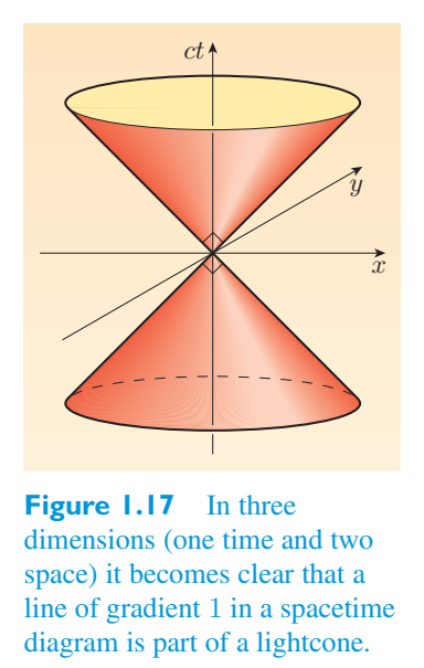
Going back to an ordinary two-dimensional spacetime diagram of the kind shown in Figure 1.18, it is straightforward to read off the coordinates of an event in frame S or in frame \(S'\). The event 1 in the diagram clearly has coordinates (ct 1, \(x^1\)) in frame S. In frame \(S'\), it has a different set of coordinates. These can be determined by drawing construction lines parallel to the lines representing the primed axes. Where a construction line parallel to one primed axis intersects the other primed axis, the coordinate can be found. By doing this on both axes, both coordinates are found. In the case of Figure 1.18, the dashed construction lines show that, as observed in frame \(S'\), event 1 occurs at the same time as event 2, and at the same position as event 3.回到图 1.18 所示的普通二维时空图,可以直接读取 S 系或 \(S'\) 系中事件的坐标。图中的事件 1 显然在 S 帧中具有坐标 (ct 1, \(x^1\))。在 \(S'\) 帧中,它具有一组不同的坐标。这些可以通过绘制与代表带底漆的轴的线平行的构造线来确定。当平行于一个主轴的构造线与另一个主轴相交时,可以找到坐标。通过在两个轴上执行此操作,可以找到两个坐标。在图 1.18 的情况下,虚线表示,如在帧 \(S'\) 中观察到的,事件 1 与事件 2 同时发生,并且与事件 3 发生在同一位置。
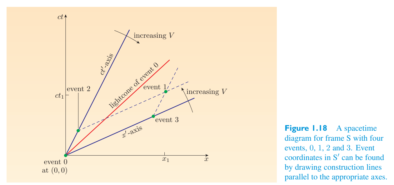
Another lesson that can be drawn from Figure 1.18 concerns the order of events. Starting from the bottom of the ct -axis and working upwards, it is clear that in frame S, the four events occur in the order 0, 2, 3 and 1. But it is equally clear from the dashed construction lines that in frame \(S'\), event 3 happens at the same time as event 0, and both happen at an earlier time than event 2 and event 1, which are also simultaneous in \(S'\). This illustrates the relativity of simultaneity, but more importantly it also shows that the order of events 2 and 3 will be different for observers O and \(O'\).从图 1.18 中可以得出的另一个教训涉及事件的顺序。从 ct 轴底部开始向上,可以清楚地看出,在帧 S 中,四个事件按 0、2、3 和 1 的顺序发生。但从虚线构造线同样可以清楚地看出,在帧 \(S'\) 中,事件 3 与事件 0 同时发生,并且两者发生的时间早于事件 2 和事件 1,而事件 2 和事件 1 在 \(S'\) 中也是同时发生的。这说明了同时性的相对性,但更重要的是,它还表明对于观察者 O 和 \(O'\) 来说,事件 2 和 3 的顺序会不同。
At first sight it is quite shocking to learn that the relative motion of two observers can reverse the order in which they observe events to happen. This has the potential to overthrow our normal notion of causality, the principle that all observers must agree that any effect is preceded by its cause. It is easy to imagine observing the pressing of a plunger and then observing the explosion that it causes. It would be very shocking, however, if some other observer, simply by moving sufficiently fast in the right direction, was able to observe the explosion first and then the pressing of the plunger that caused it. (It is important to remember that we are discussing observing, not seeing.)乍一看,两个观察者的相对运动可以颠倒他们观察事件发生的顺序,这真是令人震惊。这有可能推翻我们正常的因果关系概念,即所有观察者都必须同意任何结果都先有其原因的原则。很容易想象观察柱塞的按压,然后观察它引起的爆炸。然而,如果其他观察者仅仅通过在正确的方向上足够快地移动,能够首先观察到爆炸,然后观察到导致爆炸的柱塞的按压,那将是非常令人震惊的。 (重要的是要记住,我们正在讨论观察,而不是看到。)
Fortunately, such an overthrow of causality is not permitted by special relativity, provided that we do not allow signals to travel at speeds greater than c. Although observers will disagree about the order of some events, they will not disagree about the order of any two events that might be linked by a light signal or any signal that travels at less than the speed of light. Such events are said to be causally related.幸运的是,狭义相对论不允许这种因果关系的推翻,前提是我们不允许信号以大于 c 的速度传播。尽管观察者会对某些事件的顺序有不同意见,但他们不会对可能通过光信号或任何以低于光速传播的信号联系起来的任何两个事件的顺序有不同意见。据说这些事件是有因果关系的。
To see how the order of causally related events is preserved, look again at Figure 1.18, noting that all the events that are causally related to event 0 are contained within its lightcone, and that includes event要了解如何保留因果相关事件的顺序,请再次查看图 1.18,注意与事件 0 因果相关的所有事件都包含在其光锥内,其中包括事件
2. Events that are not2. 不存在的事件
causally related to event 0, such as event 1 and event 3, are outside the lightcone of event 0 and could only be linked to that event by signals that travel faster than light. Now, remember that as the relative speed V of the observers O and \(O'\) increases, the line representing the \(ct'\)-axis closes in on the lightcone. As a result, there will not be any value of V that allows the causally related events 0 and 2 to change their order. Event 2 will always be at a higher value of \(ct'\) than event 0. However, when you examine the corresponding behaviour of events 0 and 3, which are not causally related, the conclusion is quite different. Figure 1.18 shows the condition in which event 0 and event 3 occur at the same time \(t'\) = 0, according to \(O'\). When O and \(O'\) have a lower relative speed, event 3 occurs after event 0, but as V increases and the line representing the \(x'\)-axis (where all events occur at \(ct'\) = 0) closes in on the lightcone, we see that there will be a value of V above which the order of event 0 and event 3 is reversed.与事件 0 因果相关的事件(例如事件 1 和事件 3)位于事件 0 的光锥之外,并且只能通过传播速度快于光速的信号与该事件相关联。现在,请记住,随着观察者 O 和 \(O'\) 的相对速度 V 的增加,表示 \(ct'\) 轴的线会靠近光锥。因此,不会有任何 V 值允许因果相关的事件 0 和 2 更改其顺序。事件 2 的 \(ct'\) 值始终高于事件 0。但是,当您检查没有因果关系的事件 0 和 3 的相应行为时,结论会大不相同。图1.18显示了根据\(O'\),事件0和事件3同时发生\(t'\) = 0的情况。当 O 和 \(O'\) 的相对速度较低时,事件 3 在事件 0 之后发生,但随着 V 的增加,代表 \(x'\) 轴的线(其中所有事件发生在 \(ct'\) = 0 处)在光锥上闭合,我们看到将存在一个 V 值,高于该值时事件 0 和事件 3 的顺序相反。
So, if event 0 represents the pressing of a plunger and event 2 and event 3 represent explosions, all observers will agree that event 0 might have caused event 2, which happened later. However, those same observers will not agree about the order of event 0 and event 3, though they will agree that event 0 could not have caused event 3 unless bodies or signals can travel faster than light. It is the desire to preserve causal relationships that is the basis for the requirement that no material body or signal of any kind should be able to travel faster than light.因此,如果事件 0 代表柱塞的按压,而事件 2 和事件 3 代表爆炸,则所有观察者都会同意事件 0 可能导致了稍后发生的事件 2。然而,这些观察者不会就事件 0 和事件 3 的顺序达成一致,尽管他们会同意事件 0 不可能导致事件 3,除非物体或信号的传播速度比光快。维护因果关系的愿望是要求任何物质体或任何类型的信号都不能比光传播得更快的要求的基础。
- ● Is event 1 in Figure 1.18 causally related to event 0● 图1.18中的事件1与事件0有因果关系吗
? Is event 1 causally related to event 3? Justify your answers.?事件 1 与事件 3 有因果关系吗?证明你的答案合理。
❍ Event 1 is outside the lightcone of event 0, so the two cannot be causally related. The diagram does not show the lightcone of event 3, but if you imagine a line of gradient 1, parallel to the shown lightcone, passing through event 3, it is clear that event 1 is inside the lightcone of event 3, so those two events are causally related. The earlier event may have caused the later one, and all observers will agree about that.❍ 事件 1 在事件 0 的光锥之外,因此两者不可能存在因果关系。该图未显示事件 3 的光锥,但如果您想象一条与所示光锥平行的梯度 1 线穿过事件 3,则很明显事件 1 位于事件 3 的光锥内部,因此这两个事件存在因果关系。较早的事件可能导致了较晚的事件,所有观察者都会同意这一点。
An important lesson to learn from this question is the significance of drawing lightcones for events other than those at the origin. Every event has a lightcone, and that lightcone is of great value in determining causal relationships.从这个问题中学到的一个重要教训是,为除原点以外的事件绘制光锥的重要性。每个事件都有一个光锥,而该光锥对于确定因果关系具有很大的价值。
1.4.2 Spacetime separation and the Minkowski metric1.4.2 时空分离和闵可夫斯基度规
In three-dimensional space, the separation between two points (\(x^1\), y 1, z 1) and (\(x_{2}\), \(y^{2}\), \(z^{2}\)) can be conveniently described by the square of the distance \(\Delta l\) between them:在三维空间中,两点 (\(x^1\), y 1, z 1) 和 (\(x_{2}\), \(y^{2}\), \(z^{2}\)) 之间的间隔可以方便地用它们之间的距离 \(\Delta l\) 的平方来描述:
where \(\Delta x = x\)− x, \(\Delta y = y\)− y and \(\Delta z = z\)− z. This quantity has the useful property of being unchanged by rotations of the coordinate system. So, if we choose to describe the points using a new coordinate system with axes \(x'\), \(y'\) and \(z'\), obtained by rotating the old system about one or more of its axes, then the spatial separation of the two points would still be described by an expression of the form其中 \(\Delta x = x\)− x、\(\Delta y = y\)− y 和 \(\Delta z = z\)− z。该量具有不随坐标系旋转而改变的有用特性。因此,如果我们选择使用具有 \(x'\)、\(y'\) 和 \(z'\) 轴的新坐标系(通过绕一个或多个轴旋转旧系统而获得)来描述点,那么两个点的空间分离仍将由以下形式的表达式来描述
and we would find in addition that此外我们还会发现
We describe this situation by saying that the spatial separation of two points is invariant under rotations of the coordinate system used to describe the positions of the two points.我们通过这样的说法来描述这种情况:在用于描述两点位置的坐标系旋转的情况下,两点的空间间隔是不变的。
These ideas can be extended to four-dimensional Minkowski spacetime, where the most useful expression for the spacetime separation of two events is the following.这些想法可以扩展到四维闵可夫斯基时空,其中两个事件的时空分离最有用的表达式如下。
Spacetime separation时空分离
The reason why this particular form is chosen is that it turns out to be invariant under Lorenz transformations. So, if O and \(O'\) are inertial observers using frames S and \(S'\), they will generally not agree about the coordinates that describe two events 1 and 2, or about the distance or the time that separates them, but they will agree that the two events have an invariant spacetime separation选择这种特殊形式的原因是它在洛伦兹变换下是不变的。因此,如果 O 和 \(O'\) 是使用坐标系 S 和 \(S'\) 的惯性观察者,他们通常不会就描述两个事件 1 和 2 的坐标,或者将它们分开的距离或时间达成一致,但他们会同意这两个事件具有不变的时空分离。
Exercise 1.8 Two events occur at (ct, x, y, z) = (3, 7, 0, 0) m and练习 1.8 两个事件发生在 (ct, x, y, z) = (3, 7, 0, 0) m 处,并且
(ct, x, y, z) = (5, 5, 0, 0) m. What is their spacetime separation?(ct, x, y, z) = (5, 5, 0, 0) m。他们的时空间隔是多少?
Exercise 1.9 In the case that \(\Delta y = 0 and\)\(\Delta z = 0\), use the interval练习 1.9 在 \(\Delta y = 0\)且 \(\Delta z = 0\)的情况下,使用区间
transformation rules to show that the spacetime separation given by Equation 1.49 really is invariant under Lorentz transformations.变换规则表明方程 1.49 给出的时空分离在洛伦兹变换下确实是不变的。
A convenient way of writing the spacetime separation is as a summation:写出时空分离的一种方便方法是求和:
where the four quantities \(\Delta x\) 0, \(\Delta x\) 1, \(\Delta x\) 2 and \(\Delta x\) 3 are the components of [\(\Delta x\) \(\mu\)] = (c \(\Delta t\), \(\Delta x\), \(\Delta y\), \(\Delta z\)), and the new quantities \(\eta\) that have been introduced are the sixteen components of an entity called the Minkowski metric, which can be represented as其中,四个量 \(\Delta x\) 0、\(\Delta x\) 1、\(\Delta x\) 2 和 \(\Delta x\) 3 是 [\(\Delta x\) \(\mu\)] = (c \(\Delta t\), \(\Delta x\), \(\Delta y\), \(\Delta z\)) 的分量,引入的新量 \(\eta\) 是称为闵可夫斯基度规的实体的 16 个分量,可以表示为
It’s worth noting that the Minkowski metric has been shown as a matrix only for convenience; Equation 1.51 is not a matrix equation, though it is a well-defined sum. The important point is that the quantity [\(\eta\) \(\mu\)\(\nu\)] has sixteen components, and from Equation 1.52 you can uniquely identify each of them. The metric provides a valuable reminder of how the spacetime separation is related to the coordinate intervals. Metrics will have a crucial role to play in the rest of this book. The Minkowski metric is just the first of many that you will meet.值得注意的是,为了方便起见,将闵可夫斯基度规显示为矩阵。方程 1.51 不是一个矩阵方程,尽管它是一个明确定义的和。重要的一点是,数量 [\(\eta\) \(\mu\)\(\nu\)] 有 16 个分量,从公式 1.52 中您可以唯一地识别它们中的每一个。该度规提供了关于时空分离与坐标间隔如何相关的有价值的提醒。指标将在本书的其余部分中发挥至关重要的作用。闵可夫斯基度规只是您将遇到的众多度规中的第一个。
The spacetime separation of two events is an important quantity for several reasons. Its sign alone tells us about the possible causal relationship between the events. In fact, we can identify three classes of relationship, corresponding to the cases (\(\Delta s\)) 2 > 0, (\(\Delta s\)) 2 = 0 and (\(\Delta s\)) 2 < 0.由于多种原因,两个事件的时空间隔是一个重要的量。它的符号本身就告诉我们事件之间可能存在的因果关系。事实上,我们可以识别三类关系,分别对应于 (\(\Delta s\)) 2 > 0、(\(\Delta s\)) 2 = 0 和 (\(\Delta s\)) 2 < 0 的情况。
Time-like, light-like and space-like separations似时间、似光、似空间的分离
Events with a positive spacetime separation, (\(\Delta s\)) 2 > 0, are said to be time-like separated. Such events are causally related, and there will exist a frame in which the two events happen at the same place but at different times.具有正时空分离 (\(\Delta s\)) 2 > 0 的事件被称为类时间分离。此类事件是有因果关系的,并且会存在一个框架,其中两个事件在同一地点但不同时间发生。
s) 2 = 0, are said to be Events with a zero (or null) spacetime separation, (\(\Delta l\)ight-like separated. Such events are causally related, and all observers will agree that they could be linked by a light signal.s) 2 = 0,被认为是零(或零)时空分离的事件,(\(\Delta l\)ight-like 分离)。此类事件是因果相关的,所有观察者都会同意它们可以通过光信号联系起来。
Events with a negative spacetime separation, (\(\Delta s\)) 2 < 0, are said to be space-like separated. Such events are not causally related, and there will exist a frame in which the two events happen at the same time but at different places.具有负时空分离 (\(\Delta s\)) 2 < 0 的事件被称为类空间分离。此类事件没有因果关系,并且会存在一个框架,其中两个事件同时发生但在不同地点。
These different kinds of spacetime separation correspond to different regions of spacetime defined by the lightcone of an event. Figure这些不同类型的时空分离对应于由事件的光锥定义的不同时空区域。数字
1.19 shows the lightcone of1.19 显示了光锥
event 0. All the events that have a time-like separation from event 0 are within the future or past lightcone of event 0; all the events that are light-like separated from event 0 are on its lightcone; and all the events that are space-like separated from event 0 are outside its lightcone. This emphasizes the role that lightcones play in revealing the causal structure of Minkowski spacetime.事件 0。与事件 0 具有类似时间间隔的所有事件都在事件 0 的未来或过去光锥内;所有与事件 0 分离的类似光的事件都在其光锥上;所有与事件 0 类似空间分离的事件都在其光锥之外。这强调了光锥在揭示闵可夫斯基时空因果结构中所发挥的作用。
Another reason why spacetime separation is important relates to proper time. You will recall that in the earlier discussion of time dilation, it was said that the proper time between two events was the time separating those events as measured in a frame where the events happen at the same position. In such a frame, the spacetime separation of the events is (\(\Delta s\)) 2 = \(c^2\) (\(\Delta t\)) 2 = \(c^2\) (\(\Delta \tau\)) 2. However, since the spacetime separation of events is an invariant quantity, we can use it to determine the proper time between two time-like separated events, irrespective of the frame in which the events are described. For two time-like separated events with positive spacetime separation (\(\Delta s\)) 2, the proper time \(\Delta \tau\) between those two events is given by the following.时空分离很重要的另一个原因与原时有关。您会记得,在前面关于时间膨胀的讨论中,据说两个事件之间的固有时间是在事件发生在同一位置的帧中测量的分隔这些事件的时间。在这样的坐标系中,事件的时空间隔为 (\(\Delta s\)) 2 = \(c^2\) (\(\Delta t\)) 2 = \(c^2\) (\(\Delta \tau\)) 2。然而,由于事件的时空分离是一个不变的量,我们可以用它来确定两个类似时间的分离事件之间的固有时间,而不管事件描述的框架如何。对于两个具有正时空间隔 (\(\Delta s\)) 2 的类时分离事件,这两个事件之间的本征时间 \(\Delta \tau\) 由下式给出。
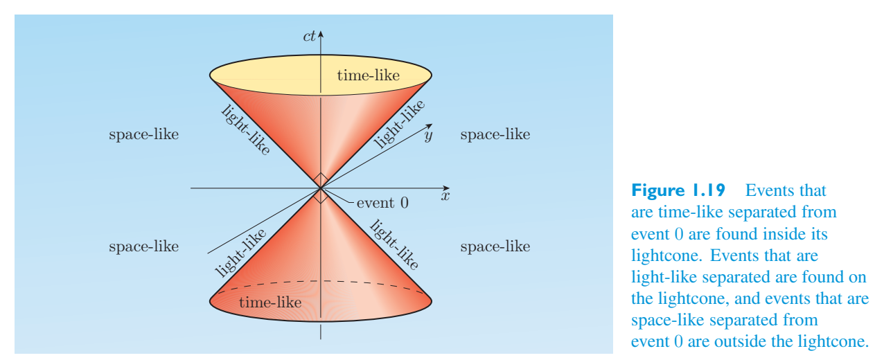
Proper time related to spacetime separation与时空分离相关的本征时间
The relation between proper time and the invariant spacetime separation is extremely useful in special relativity. The reason for this relates to the length of a particle’s pathway through four-dimensional Minkowski spacetime. Such a pathway, with all its twists and turns, records the whole history of the particle and is sometimes called its world-line. (One well-known relativist called his autobiography My worldline.) By adding together the spacetime separations between successive events along a particle’s world-line, and dividing the sum by \(c^2\), we can determine the total time that has passed according to a clock carried by the particle. This simple principle will be used to help to explain a troublesome relativistic effect in the next subsection.原时与不变时空分离之间的关系在狭义相对论中极其有用。其原因与粒子穿过四维闵可夫斯基时空的路径长度有关。这样一条充满曲折的路径记录了粒子的整个历史,有时被称为它的世界线。(一位著名的相对论者将他的自传称为“我的世界线”。)通过将粒子世界线上连续事件之间的时空间隔相加,并将总和除以 \(c^2\),我们可以根据粒子携带的时钟确定已经过去的总时间。这个简单的原理将用于帮助解释下一小节中麻烦的相对论效应。
In this book, a positive sign will always be associated with the square of the time interval in the spacetime separation, and a negative sign with the spatial intervals. This choice of sign is just a convention, and the opposite set of signs could have been used. The convention used here ensures that the spacetime separation of events on the world-line of an object moving slower than light is positive. Nonetheless, you will find that many authors adopt the opposite convention, so when consulting other works, always pay attention to the sign convention that they are using.在本书中,正号总是与时空间隔中的时间间隔的平方相关联,而负号则与空间间隔相关联。这种符号选择只是一种惯例,也可以使用相反的符号集。这里使用的约定确保运动速度慢于光的物体的世界线上事件的时空分离是正的。尽管如此,你会发现许多作者采用相反的约定,因此在查阅其他作品时,请始终注意他们使用的符号约定。
Exercise 1.10 Given two time-like separated events, show that the proper time练习 1.10 给定两个类似时间的分离事件,证明适当的时间
between those events is the least amount of time that any observer will measure between them.这些事件之间的间隔是任何观察者在它们之间测量的最短时间。
1.4.3 The twin effect1.4.3 孪生效应
We end this chapter with a discussion of a well-known relativistic effect, the twin effect. This caused a great deal of controversy early in the theory’s history. It is usually presented as a thought experiment concerning the phenomenon of time dilation. The thought experiment involves two twins, Astra and Terra. The twins are identical in every way, except that Astra likes to travel around very fast in her spaceship, while Terra prefers to stay at home on Earth.我们以对著名的相对论效应——孪生效应的讨论来结束本章。这在该理论的历史早期引起了很大的争议。它通常表现为关于时间膨胀现象的思想实验。这个思想实验涉及两个双胞胎,阿斯特拉和泰拉。这对双胞胎在各方面都完全相同,只是阿斯特拉喜欢在她的宇宙飞船中快速旅行,而泰拉更喜欢呆在地球上的家里。
As was demonstrated earlier in this chapter, fast-moving objects are subject to observable time dilation effects. This indicates that if Astra jets off in some fixed direction at close to the speed of light, then, as measured by Terra, she will age more slowly because ‘moving clocks run slow’. This is fine — it is just what relativity theory predicts, and agrees with the observed behaviour of high-speed particles. But now suppose that Astra somehow manages to turn around and return to Earth at equally high speed. It seems clear that Terra will again observe that Astra’s clock will run slow and will therefore not be surprised to find that on her return, Astra has aged less than her stay-at-home twin Terra.正如本章前面所演示的,快速移动的物体会受到可观察到的时间膨胀效应的影响。这表明,如果阿斯特拉以接近光速的速度向某个固定方向喷射,那么根据泰拉的测量,她的衰老速度会更慢,因为“移动的时钟走得很慢”。这很好——这正是相对论的预测,并且与观察到的高速粒子的行为一致。但现在假设阿斯特拉以某种方式设法转身并以同样高的速度返回地球。很明显,泰拉将再次观察到阿斯特拉的时钟会变慢,因此不会惊讶地发现,在她回来时,阿斯特拉的年龄比她待在家里的双胞胎泰拉要小。
The supposed problem arises when this process is examined from Astra’s point of view. Would it not be the case, some argued, that Astra would observe the same events apart from a reversal of velocities, so that Terra would be the travelling twin and it would be Terra’s clock that would be running slow during both parts of the journey? Consequently, shouldn’t Astra expect Terra to be the younger when they were reunited? Clearly, it’s not possible for each twin to be younger than the other when they meet at the same place, so if the arguments are equally sound, it was said, there must be something wrong with special relativity.当从 Astra 的角度审视这个过程时,就会出现所谓的问题。一些人认为,除了速度逆转之外,阿斯特拉是否会观察到相同的事件,因此泰拉将是旅行的双胞胎,而泰拉的时钟在旅程的两个部分都会变慢?因此,阿斯特拉不应该期望泰拉在他们重聚时变得更年轻吗?显然,当双胞胎在同一个地方相遇时,他们不可能比另一个年轻,所以如果论证同样合理,有人说,狭义相对论一定有问题。
In fact, the arguments are not equally sound. The basic problem is that the presumed symmetry between Terra’s view and Astra’s view is illusory. It is Astra who would be the younger at the reunion, as will now be explained with the aid of a spacetime diagram and a proper use of spacetime separations in Minkowski space.事实上,这些论点并不同样合理。基本问题是,泰拉的视图和阿斯特拉的视图之间假定的对称性是虚幻的。阿斯特拉在重聚时将是更年轻的,现在将借助时空图和正确使用闵可夫斯基空间中的时空分离进行解释。
The first point to make clear is that although velocity is a purely relative quantity, acceleration is not. According to the first postulate of special relativity, the laws of physics do not distinguish one inertial frame from another, so a traveller in a closed box cannot determine his or her speed by performing a physics experiment. However, such a traveller would certainly be able to feel the effect of any acceleration, as we all know from everyday experience. In order to leave the Solar System, jet around the galaxy and return, Astra must have undergone a change in velocity, and that would involve a detectable acceleration. To a first approximation, Terra does not accelerate (her velocity changes due to the rotation and revolution of the Earth are very small compared with Astra’s accelerations). A single inertial frame of reference is sufficient to represent Terra’s view of events, but no single inertial frame can adequately represent Astra’s view. There is no symmetry between these two observers; only Terra is an (approximately) inertial observer.首先要明确的是,虽然速度是一个纯粹的相对量,但加速度却不是。根据狭义相对论第一假设,物理定律无法区分一个惯性系和另一个惯性系,因此封闭盒子中的旅行者无法通过进行物理实验来确定他或她的速度。然而,正如我们从日常经验中知道的那样,这样的旅行者肯定能够感受到任何加速度的影响。为了离开太阳系,绕银河系喷射并返回,阿斯特拉必须经历速度变化,这将涉及可检测到的加速度。初步估计,Terra 并没有加速(与 Astra 的加速度相比,她因地球自转和公转而产生的速度变化非常小)。单一惯性参考系足以代表泰拉对事件的看法,但没有单一惯性系能够充分代表阿斯特拉的观点。这两个观察者之间不存在对称性;只有 Terra 是(近似)惯性观察者。
In order to be clear about what’s going on and to avoid the use of non-inertial frames, it is convenient to use three inertial frames when discussing the twin effect. The first is Terra’s frame, which we can treat as fixed on a non-rotating, non-revolving Earth. The second, which we shall call Astra’s frame, moves at a high but constant speed V relative to Terra’s frame. You can think of this as the frame of Astra’s spaceship, and you can think of Astra as simply jumping aboard her passing ship at the departure, event 0, when she leaves Terra to begin the outward leg of her journey. The third inertial frame, called Stella’s frame, belongs to another space traveller who happens to be approaching Earth at speed V along the same line that Astra leaves along. At some point, Stella’s ship will pass Astra’s, and at that point we can imagine that Astra jumps from her ship to Stella’s ship to make the return leg of her journey. Of course, this is unrealistic since the ‘jump’ would kill Astra, so you may prefer to imagine that Astra is actually a conscious robot or even that she can somehow ‘teleport’ from one ship to another. In any case, the important point is that the transfer is abrupt and has no effect on Astra’s age.为了清楚地了解发生了什么并避免使用非惯性系,在讨论孪生效应时可以方便地使用三个惯性系。第一个是 Terra 的框架,我们可以将其视为固定在不自转、不公转的地球上。第二个,我们称之为阿斯特拉框架,相对于泰拉框架以高但恒定的速度 V 移动。您可以将其视为阿斯特拉宇宙飞船的框架,并且您可以将阿斯特拉视为简单地在事件 0 出发时跳上她经过的飞船,当她离开泰拉开始她的旅程的向外旅程时。第三个惯性系,称为斯特拉系,属于另一位太空旅行者,他恰好沿着阿斯特拉离开的同一条线以速度 V 接近地球。在某个时刻,斯特拉的船将经过阿斯特拉的船,那时我们可以想象阿斯特拉从她的船上跳到斯特拉的船上,开始她的旅程的回程。当然,这是不现实的,因为“跳跃”会杀死阿斯特拉,所以你可能更愿意想象阿斯特拉实际上是一个有意识的机器人,甚至她可以以某种方式从一艘船“传送”到另一艘船。无论如何,重要的一点是,转会是突然的,对阿斯特拉的年龄没有影响。
The event at which Astra makes the transfer to Stella’s ship we shall call event 1, and the event at which Astra and Terra are eventually reunited we shall call event 2. Astra’s quick transfer from one ship to the other allows us to discuss the essential features of the twin effect without getting bogged down in details about the nature of the acceleration that Astra experiences. It is vital that Astra is accelerated, but exactly how that happens is unimportant. Note that we may treat each of these frames as being in standard configuration with either of the others. We can set up the frames in such a way that the origins of Terra’s frame and Astra’s frame coincide at event 0, the origins of Astra’s frame and Stella’s frame coincide at event 1, and the origins of Stella’s frame and Terra’s frame coincide at event 2.阿斯特拉转移到斯特拉飞船的事件我们称为事件 1,而阿斯特拉和泰拉最终团聚的事件我们称为事件 2。阿斯特拉从一艘船快速转移到另一艘船使我们能够讨论双生效应的基本特征,而不必陷入有关阿斯特拉所经历的加速性质的细节。Astra 的加速至关重要,但具体如何发生并不重要。请注意,我们可以将这些框架中的每一个视为与其他框架中的任何一个的标准配置。我们可以这样设置框架,使得 Terra 框架和 Astra 框架的原点在事件 0 处重合,Astra 框架和 Stella 框架的原点在事件 1 处重合,Stella 框架和 Terra 框架的原点在事件 2 处重合。
Figure 1.20 is a spacetime diagram for Terra’s frame, showing all these events and making clear the coordinates that Terra assigns to them.图1.20是Terra框架的时空图,显示了所有这些事件并明确了Terra分配给它们的坐标。
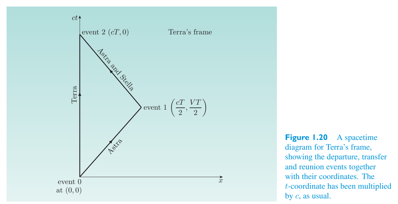
It is clear from the figure that the proper time between departure and reunion (both of which happen at Terra’s location) is T. A little calculation using the relation (\(\Delta \tau\)) 2 = (\(\Delta s\)) 2/\(c^2\) makes it equally clear that the proper time between event 0 and event 1 is given by从图中可以清楚地看出,出发和团聚(两者都发生在 Terra 所在位置)之间的正确时间为 T。使用关系式 (\(\Delta \tau\)) 2 = (\(\Delta s\)) 2/\(c^2\) 进行一点计算,同样可以清楚地看出,事件 0 和事件 1 之间的正确时间由下式给出:
So所以
Although we have arrived at this result using the coordinates assigned by Terra, it is important to note that proper time is an invariant, so all inertial observers will agree on the proper time between two events no matter how it is calculated.虽然我们是使用 Terra 指定的坐标得出这个结果,但值得注意的是,原时是一个不变量,因此所有惯性观察者都会就两个事件之间的原时达成一致,无论它是如何计算的。
A similar calculation for the proper time separating event对固有时间分隔事件的类似计算
So the total proper time that elapses along the world-line followed by Astra is \(\Delta \tau\) 0, 1 + \(\Delta \tau\) 1, 2 = T/γ. As expected, this shows that Astra will be the younger twin at the time of the reunion.因此,阿斯特拉沿世界线经过的总固有时间为 \(\Delta \tau\) 0, 1 + \(\Delta \tau\) 1, 2 = T/γ。不出所料,这表明阿斯特拉将成为重聚时的双胞胎中的弟弟。
How is it possible for Terra and Astra to disagree about the proper time between events 0 and 2? The answer to this question is that when the whole trip is considered, Astra is not an inertial observer; she undergoes an acceleration that Terra does not.Terra 和 Astra 怎么可能在事件 0 和 2 之间的正确时间上存在分歧?这个问题的答案是,当考虑整个行程时,Astra并不是一个惯性观察者;而是一个惯性观察者。她经历了泰拉没有经历的加速。
The analysis that we have just completed is really sufficient to settle any questions about the twin effect. However, it is still instructive to examine the same events from Astra’s frame (which she leaves at event 1). The spacetime diagram for Astra’s frame is shown in Figure 1.21. The coordinates of the events have been worked out from those given in Terra’s frame using the Lorentz transformations.我们刚刚完成的分析确实足以解决有关孪生效应的任何问题。然而,从阿斯特拉的框架中检查相同的事件(她在事件 1 中留下)仍然具有启发性。 Astra 框架的时空图如图 1.21 所示。事件的坐标是使用洛伦兹变换根据 Terra 框架中给出的坐标计算出来的。
- ● Confirm the coordinate assignments shown in Figure● 确认如图所示的坐标分配
1.21.1.21。
❍ In Terra’s frame, event 0 is at (ct, x) = (0, 0), event 1 at (cT/2, V T/2), and event 2 at (cT, 0). Treating Terra’s frame as frame S and Astra’s frame as \(S'\), and using the Lorentz transformations \(t'\) = \(\gamma(t - V x/\(c^2\))\) and \(x'\) = \(\gamma(x - V t)\), it follows immediately that in Astra’s frame, event 0 is at (\(ct'\), \(x'\)) = (0, 0), event 1 is at (\(ct'\), \(x'\)) = (cT/2 γ, 0) (remember that \(\gamma(V)\) = 1/1 − \(V^{2}\)/\(c^2\)), and event 2 is at (\(ct'\), \(x'\)) = (cγT, − γV T).❍ 在 Terra 的框架中,事件 0 位于 (ct, x) = (0, 0),事件 1 位于 (cT/2, V T/2),事件 2 位于 (cT, 0)。将 Terra 的坐标系视为坐标系 S,将 Astra 的坐标系视为 \(S'\),并使用洛伦兹变换 \(t'\) = \(\gamma(t - V x/\(c^2\))\) 和 \(x'\) = \(\gamma(x - V t)\),紧接着可以得出在 Astra 的坐标系中,事件 0 位于 (\(ct'\), \(x'\)) = (0, 0),事件 1 位于 (\(ct'\), \(x'\)) = (cT/2 γ, 0)(记住 \(\gamma(V)\) = 1/1 − \(V^{2}\)/\(c^2\)),事件 2 位于 (\(ct'\), \(x'\)) = (cγT, − γV T)。
Note that again there is a kink in Astra’s world-line due to the acceleration that she undergoes. There is no such kink in Terra’s world-line since she is an inertial observer. Once again we can work out the proper time that Astra experiences while passing between the three events: this represents the time that would have elapsed according to a clock that Astra carries between each of the events. The, 1 = T/2 γ, since those proper time between event 0 and event 1 is simply \(\Delta \tau\) 0 events happen at the same place in Astra’s frame. The proper time between event 1 and event 2 is given by请注意,由于阿斯特拉经历的加速,她的世界线再次出现了扭结。泰拉的世界线中不存在这样的扭结,因为她是惯性观察者。我们可以再次计算出阿斯特拉在这三个事件之间经过时所经历的正确时间:这代表根据阿斯特拉在每个事件之间携带的时钟所经过的时间。1 = T/2 γ,因为事件 0 和事件 1 之间的正确时间就是 \(\Delta \tau\) 0 个事件发生在 Astra 框架中的同一位置。事件 1 和事件 2 之间的正确时间由下式给出
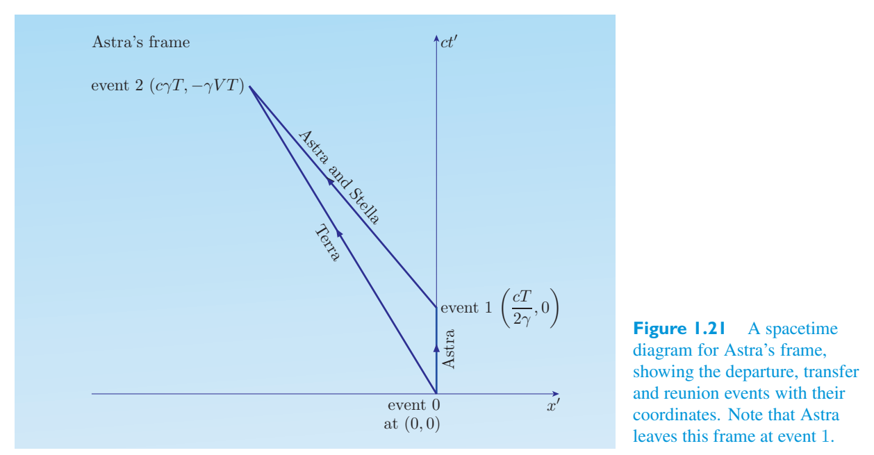
Since γ 2 (1 − \(V^{2}\)/\(c^2\)) = 1, the above expression simplifies to give由于 γ 2 (1 − \(V^{2}\)/\(c^2\)) = 1,上述表达式简化为
So once again the theory predicts that the time for the round trip recorded by Astra is \(\Delta \tau +\)\(\Delta \tau = T\)/γ.因此理论再次预测Astra记录的往返时间为Δτ+\(\Delta\tau=T\)/γ。
There is one other point to notice using Astra’s frame. Time dilation tells us that, as measured in Astra’s frame, Terra’s clock will be running slow. From Astra’s frame, a 1 -second tick of Terra’s clock will be observed to last γ seconds. But in Astra’s frame, it is also the case that the time of the reunion is γT, which is greater than the time of the reunion as observed in Terra’s frame. According to an observer who uses Astra’s frame, this longer journey time compensates for the slower ticking of Terra’s clock, with the result that such an observer will fully expect Terra to have aged by T while Astra herself has aged by only T/γ. Using the coordinates of event 0 and event 2 in Astra’s frame, it is easy to confirm that the proper time between them is T, which is another way of stating the same result.使用Astra 的框架还有一点需要注意。时间膨胀告诉我们,按照阿斯特拉的坐标系测量,泰拉的时钟将会走慢。从 Astra 的坐标系中,可以观察到 Terra 时钟的 1 秒滴答持续 γ 秒。但在阿斯特拉的框架中,团聚的时间也是γT,大于在泰拉的框架中观察到的团聚的时间。根据一位使用阿斯特拉框架的观察者的说法,更长的旅程时间补偿了泰拉时钟较慢的滴答声,结果是这样的观察者完全预计泰拉已经老化了 T,而阿斯特拉本身只老化了 T/γ。使用Astra框架中事件0和事件2的坐标,很容易确认它们之间的正确时间是T,这是陈述相同结果的另一种方式。
Exercise 1.11 Using the velocity transformation, show练习1.11 使用速度变换,显示
that Astra observes the \(V^{2}\)/\(c^2\)). speed of approach of Stella’s spaceship to be 2 V/(1 +Astra 观察到 \(V^{2}\)/\(c^2\))。斯特拉飞船的接近速度为 2 V/(1 +
Exercise 1.12 Suppose that Terra sends regular time练习1.12 假设Terra发送固定时间
signals towards Astra and Stella at one-second intervals. Write down expressions for the frequency at which Astra receives the signals on the outward and return legs of her journey.每隔一秒向阿斯特拉和斯特拉发出信号。写下阿斯特拉在去程和回程旅程中接收信号的频率表达式。
Summary of Chapter 1第 1 章总结
1. Basic terms in the vocabulary of relativity include:1. 相对论词汇中的基本术语包括:
event, frame of reference, inertial frame and observer.事件、参考系、惯性系和观察者。
2. A theory of relativity concerns the relationships between2. 相对论关注的是之间的关系
observations made by observers in a specified state of relative motion. Special relativity is essentially restricted to inertial observers in uniform relative motion.观察者在特定的相对运动状态下所做的观察。狭义相对论本质上仅限于匀速相对运动的惯性观察者。
3. Einstein based special relativity on two postulates:3. 爱因斯坦将狭义相对论建立在两个假设之上:
the principle of relativity (that the laws of physics can be written in the same form in all inertial frames) and the principle of the constancy of the speed of light (that all inertial observers agree that light travels through empty space with the same fixed speed, c, in all directions).相对论原理(物理定律可以在所有惯性系中以相同的形式写出)和光速恒定原理(所有惯性观察者都同意光以相同的固定速度 c 在各个方向穿过真空)。
4. Given two inertial frames S and \(S'\) in standard configuration,4. 给定标准配置的两个惯性系S和\(S'\),
the coordinates of an event observed in frame S are related to the coordinates of the same event observed in frame \(S'\) by the Lorentz transformations通过洛伦兹变换,在坐标系 S 中观察到的事件的坐标与在坐标系 \(S'\) 中观察到的同一事件的坐标相关
where the Lorentz factor is其中洛伦兹因子是
These transformations may also be represented by matrices,这些变换也可以用矩阵表示,
or as a set of summations或作为一组求和
5. The inverse Lorentz transformations may be written5.洛伦兹逆变换可以写成
as作为
6. Similar equations describe the transformation of intervals, \(\Delta t\), \(\Delta x\), etc.,6.类似的方程描述了区间、\(\Delta t\)、\(\Delta x\)等的变换,
between the two frames.两个框架之间。
7. The consequences of special relativity, deduced by considering the7. 狭义相对论的后果,通过考虑
transformation of events and intervals, include the following.事件和间隔的转换,包括以下内容。
(a) Time dilation:(a) 时间膨胀:
(b) Length contraction:(b) 长度收缩:
(c) The relativity of simultaneity.(c)同时性的相对性。
(c + V)/(c − V) (for an approaching source),(c + V)/(c − V)(对于接近源),
(c − V)/(c + V) (for a receding source).(c − V)/(c + V)(对于后退源)。
(e) The velocity transformation:(e) 速度变换:
8. Four-dimensional Minkowski spacetime contains all possible events.8. 四维闵可夫斯基时空包含所有可能的事件。
9. Spacetime diagrams showing events as observed by a particular observer are9. 显示特定观察者观察到的事件的时空图是
a valuable tool that can provide pictorial insights into relativistic effects and the structure of Minkowski spacetime.这是一个有价值的工具,可以为相对论效应和闵可夫斯基时空结构提供图形化的见解。
10. Lightcones are particularly useful for understanding causal relationships10.光锥对于理解因果关系特别有用
between events in Minkowski spacetime.闵可夫斯基时空中的事件之间。
11. The invariant spacetime separation between two events has the form11. 两个事件之间的不变时空间隔具有以下形式
and may be positive (time-like), zero (light-like) or negative (space-like).并且可以是正值(类时间)、零(类光)或负值(类空间)。
12. The spacetime separation may be conveniently written as12. 时空分离可以方便地写为
where the \(\eta\) \(\mu\)\(\nu\) are the components of the Minkowski metric其中 \(\eta\) \(\mu\)\(\nu\) 是闵可夫斯基度规的组成部分
13. The proper time \(\Delta \tau\) between two time-like separated13. 两个类似时间间隔之间的正确时间\(\Delta \tau\)
events is given by事件由下式给出
This is the time that would be recorded on a clock that moves uniformly between the two events.这是记录在两个事件之间均匀移动的时钟上的时间。
14. The proper time between two events is an invariant14. 两个事件之间的固有时间是一个不变量
under Lorentz transformations.在洛伦兹变换下。
Chapter 2 Special relativity and physical laws第二章狭义相对论和物理定律
Introduction介绍
Physical laws are usually expressed mathematically, as equations. They are used by physicists to summarize their findings regarding the basic principles that govern the Universe. From the late 1600s to the mid-1800s, Newton’s laws and the Galilean relativity underpinning them were believed to be the fundamental rules. The precision engineering of the nineteenth century and the clock-like regularity of the Solar System all seemed to be consistent with this view.物理定律通常以数学形式表达为方程。物理学家用它们来总结他们关于支配宇宙的基本原理的发现。从 1600 年代末到 1800 年代中期,牛顿定律和支撑牛顿定律的伽利略相对论被认为是基本规则。十九世纪的精密工程和太阳系的时钟般的规律性似乎都与这一观点相一致。
However, as we have already seen, the investigation of electricity and magnetism, and their unification with optics through Maxwell’s demonstration of the electromagnetic nature of light, exposed a new conflict between fundamental laws. Lorentz and others worked on this problem but it was Einstein who recognized most clearly and completely that its essence was in a conflict between the invariance of the speed of light in a vacuum and the requirement of Galilean relativity that observers in relative motion should disagree about the speed of light. Einstein’s response was to extend the principle of relativity from the laws of mechanics to all the laws of physics, including specifically the constancy of the speed of light, and to accept as a consequence the need for a new theory of relativity based on the Lorentz transformations rather than Galilean transformations.然而,正如我们已经看到的,对电和磁的研究,以及通过麦克斯韦对光的电磁性质的论证,它们与光学的统一,暴露了基本定律之间的新冲突。洛伦兹和其他人致力于研究这个问题,但爱因斯坦最清楚、最彻底地认识到,其本质是真空中光速不变性与伽利略相对论的要求(即相对运动的观察者对光速的看法应该不一致)之间的冲突。爱因斯坦的回应是将相对论原理从力学定律扩展到所有物理定律,特别是光速恒定性,并因此接受基于洛伦兹变换而不是伽利略变换的新相对论的需要。
The requirement of special relativity, that physical laws should take the same form in all inertial frames, is highly restrictive. It prevents many candidates from being accepted as genuine physical laws. The principle of relativity cannot tell us which proposed laws are correct — that must be done by experiment — but it can show up those that are not acceptable in principle. When the coordinates used in two different frames are related by the Lorentz transformations, it is soon seen that the laws of Newtonian mechanics do not take the same form in all inertial frames. So an immediate implication of special relativity is the need for an extensive rewriting of the laws of mechanics. The new laws must be consistent with the well-established successes of Newtonian mechanics, but they must also show the invariance under Lorentz transformations required by the principle of relativity. In this chapter we shall consider those new laws of mechanics and see the extent to which Newtonian concepts had to be modified or replaced. We shall then go on to see what special relativity has to say about the laws of electricity and magnetism.狭义相对论的要求,即物理定律在所有惯性系中应采取相同的形式,是高度限制性的。它阻止了许多候选人被接受为真正的物理定律。相对性原理不能告诉我们哪些提出的定律是正确的——这必须通过实验来完成——但它可以显示那些原则上不可接受的定律。当两个不同框架中使用的坐标通过洛伦兹变换相关联时,很快就会发现牛顿力学定律在所有惯性系中并不采用相同的形式。因此,狭义相对论的直接含义是需要对力学定律进行广泛的重写。新定律必须与牛顿力学的既定成功相一致,但它们也必须显示相对论原理所需的洛伦兹变换下的不变性。在本章中,我们将考虑这些新的力学定律,并了解牛顿概念必须修改或替换的程度。然后我们将继续看看狭义相对论对电和磁定律的解释。
The discussion of physical laws in this chapter will introduce some important mathematical entities that may be new to you. These entities, called four-vectors and four-tensors, are of particular relevance to special relativity but they set the scene for the introduction of more general tensors in the later chapters that deal with general relativity. Pay special attention to these four-vectors and four-tensors. Appreciating their role in the formulation of physical laws that are consistent with special relativity is at least as important as learning about any specific feature of those laws.本章中对物理定律的讨论将介绍一些对您来说可能是新的重要数学实体。这些实体被称为四向量和四张量,与狭义相对论特别相关,但它们为后面讨论广义相对论的章节中引入更一般的张量奠定了基础。特别注意这四矢量量量和四个张量。理解它们在制定符合狭义相对论的物理定律中的作用至少与了解这些定律的任何具体特征一样重要。
2.1 Invariants and physical laws2.1 不变量和物理定律
2.1.1 The invariance of physical quantities2.1.1 物理量的不变性
Central to the formulation of physical laws in special relativity are invariant quantities or invariants for short. You have already met a number of these invariants: most obviously, the speed of light in a vacuum, but also the spacetime separation between events (\(\Delta s\)) 2 = (c \(\Delta t\)) 2 − (\(\Delta x\)) 2 − (\(\Delta y\)) 2 − (\(\Delta z\)) 2 and, in the case of time-like separated events, the closely related proper time interval \(\Delta \tau\) given by (\(\Delta \tau\)) 2 = (\(\Delta s\)) 2/\(c^2\).狭义相对论中物理定律表述的核心是不变量或简称不变量。您已经遇到了许多这样的不变量:最明显的是真空中的光速,还有事件之间的时空间隔 (\(\Delta s\)) 2 = (c \(\Delta t\)) 2 − (\(\Delta x\)) 2 − (\(\Delta y\)) 2 − (\(\Delta z\)) 2 以及在类似时间的分离事件的情况下,紧密相关的本征时间间隔 \(\Delta \tau\) 由 (\(\Delta \tau\)) 2 = (\(\Delta s\)) 给出2/\(c^2\)。
An alternative way of defining the proper time between two events is as the time between those events measured in a frame in which the two events occur at the same spatial position. (The fact that the events are time-like separated guarantees that such a frame exists.) This is an interesting definition since it uses a measurement made in one inertial frame to define a quantity that can then be used in all inertial frames. This approach to defining invariants is quite common. For example, we can and will say that the electric charge of a particle is the charge that it has when measured in the frame in which the particle is at rest. The charge is then defined in an invariant way, even though the prescription for measuring it involves a particular frame — the rest frame of the particle.定义两个事件之间的固有时间的另一种方法是在两个事件发生在同一空间位置的帧中测量的这些事件之间的时间。 (事件是类似时间的分离这一事实保证了这样一个框架的存在。)这是一个有趣的定义,因为它使用在一个惯性系中进行的测量来定义一个可以在所有惯性系中使用的量。这种定义不变量的方法很常见。例如,我们可以并且会说,粒子的电荷是在粒子静止的框架中测量时所具有的电荷。然后以不变的方式定义电荷,即使测量它的规定涉及特定的框架——粒子的其余框架。
A similar approach can be used to provide an invariant value for the mass of a particle. In keeping with the common practice of particle physicists, we shall say that the mass of a particle is the mass that would be measured in a frame in which the particle is at rest. This provides a mass that all observers can agree about. Some authors refer to this quantity as the rest mass of the particle, but we have no need to do so here since this is the only sense in which we shall use the term mass in this chapter. Incidentally, if you have studied relativity before, you may have encountered the idea of a relativistic mass that increases with the speed of the particle. This is based on a quite different definition of mass that will not be used in this book. The masses that we shall refer to are defined invariantly and will never depend on speed. Other invariant quantities — some of them very important — will be introduced later, but for the moment here is a summary of what we have said about invariants.可以使用类似的方法来提供粒子质量的不变值。根据粒子物理学家的惯例,我们应该说粒子的质量是在粒子静止的框架中测量的质量。这提供了所有观察者都同意的质量。一些作者将这个量称为粒子的剩余质量,但我们在这里没有必要这样做,因为这是我们在本章中使用术语“质量”的唯一含义。顺便说一句,如果您以前研究过相对论,您可能遇到过相对论质量随粒子速度增加而增加的想法。这是基于一个完全不同的质量定义,本书中不会使用该定义。我们所提到的质量是恒定定义的,并且永远不会依赖于速度。其他不变量(其中一些非常重要)将在稍后介绍,但目前这里是我们关于不变量所说的内容的总结。
Invariants不变量
An invariant is a quantity that has the same value in all inertial frames.不变量是在所有惯性系中具有相同值的量。
Invariant quantities include:不变量包括:
- • the speed of light in a vacuum, c• 真空中的光速,c
- • the spacetime separation (\(\Delta s\)) 2 = (c \(\Delta t\)) 2 − (Δ• 时空间隔 (\(\Delta s\)) 2 = (c \(\Delta t\)) 2 − (Δ
- • the proper time (\(\Delta \tau\)) 2 = (\(\Delta s\)) 2/\(c^2\) between time-like• 类时间之间的固有时间 (\(\Delta \tau\)) 2 = (\(\Delta s\)) 2/\(c^2\)
separated events分开的事件
- • the charge of a particle, q• 粒子的电荷,q
- • the mass of a particle, m.• 粒子的质量,m。
2.1.2 The invariance of physical laws2.1.2 物理定律的不变性
The requirement that the laws of physics should take the same form in all inertial frames involves extending the idea of invariance from invariance of a quantity to invariance of the form of an equation. The easiest way to appreciate this is by means of an example so, although it is mainly of historical interest, we shall now demonstrate the form invariance of Newton’s laws of motion under the Galilean coordinate transformation.物理定律在所有惯性系中应采用相同形式的要求涉及将不变性的概念从量的不变性扩展到方程形式的不变性。理解这一点的最简单方法是通过一个例子,尽管它主要具有历史意义,但我们现在将证明牛顿运动定律在伽利略坐标变换下的形式不变性。
Newton’s laws of motion can be stated as follows.牛顿运动定律可以表述如下。
1. A body maintains a constant velocity unless acted upon by an unbalanced1. 除非受到不平衡力的作用,否则物体保持恒定速度
external force.外力。
2. A body acted upon by an unbalanced force accelerates in the direction of2. 物体受到不平衡力的作用时,沿下列方向加速:
that force at a rate that is proportional to the force and inversely proportional to the body’s mass.该力的速率与力成正比,与身体质量成反比。
3. When body A exerts a force on body B, body B exerts a force on body A3.当A体对B体施加力时,B体也对A体施加力
that has the same magnitude but acts in the opposite direction. (This law is often stated as: to every action there is an equal and opposite reaction.)其大小相同,但作用方向相反。 (这条定律通常被表述为:每一个动作都会有一个相等且相反的反应。)
The first law is really telling us that in order to use the other laws, we should make sure that we observe from an inertial frame of reference. So we don’t need to give any further thought to this law as long as we restrict ourselves to inertial frames. The third law also presents no difficulty. Provided that oppositely directed forces of equal magnitude transform in the same way in Galilean relativity, there will not be any problem about agreeing on the form of the third law. This is true even for forces that act at a distance, such as the gravitational force acting on a person due to the Earth and the reaction to that force that acts simultaneously at the Earth’s centre of mass.第一定律实际上告诉我们,为了使用其他定律,我们应该确保我们从惯性参考系进行观察。因此,只要我们将自己限制在惯性系中,就无需进一步考虑该定律。第三定律也没有什么困难。假设伽利略相对论中方向相反、大小相等的力以同样的方式变换,那么就第三定律的形式达成一致就不会有任何问题。即使对于远距离作用的力也是如此,例如由于地球而作用在人身上的引力以及同时作用在地球质心的该力的反作用力。
The real challenge comes with Newton’s second law of motion. Let’s start by writing the second law as an equation真正的挑战来自牛顿第二运动定律。让我们首先将第二定律写成方程
where f is the applied force, m is the mass of the body, and a is its acceleration. If we take this to be the form of Newton’s second law in some particular inertial frame S with Cartesian coordinate axes x, y and z, we can relate the acceleration to the coordinates of the body in frame S by writing其中 f 是施加的力,m 是物体的质量,a 是物体的加速度。如果我们将其视为具有笛卡尔坐标轴 x、y 和 z 的特定惯性系 S 中牛顿第二定律的形式,我们可以将加速度与 S 系中物体的坐标联系起来:
Now suppose that we have a second frame of reference \(S'\) in standard configuration with S, so that the coordinates in the two frames are related by the Galilean transformations现在假设我们有第二个参考系 \(S'\),其标准配置为 S,因此两个参考系中的坐标通过伽利略变换相关
Differentiating the expressions for the position coordinates twice with respect to \(t'\), and noting that this is equivalent to differentiating with respect to t (since \(t'\) = t), we see that对位置坐标的表达式关于 \(t'\) 进行两次微分,并注意这相当于对 t 进行微分(因为 \(t'\) = t),我们看到
Mass is certainly an invariant in Galilean relativity, so, under a Galilean transformation from frame S to frame \(S'\), the right-hand side of Equation 2.2 becomes质量在伽利略相对论中当然是一个不变量,因此,在从 S 系到 \(S'\) 系的伽利略变换下,方程 2.2 的右侧变为
where the quantity \(a'\) has been introduced to emphasize the form-invariance of the right-hand side of Newton’s second law under a Galilean transformation. This is a promising start, but what about the left-hand side: how does the force f transform under a Galilean transformation? To answer that question, we need to know how the force depends on the coordinates.其中引入量 \(a'\) 是为了强调伽利略变换下牛顿第二定律右侧的形式不变性。这是一个充满希望的开始,但左边呢:力 f 在伽利略变换下如何变换?要回答这个问题,我们需要知道力如何取决于坐标。
For the sake of definiteness, let’s consider the case in which a body of mass m at position r = (x, y, z) is acted upon by a gravitational force due to a body of mass M at position R = (X, Y, Z) (see Figure 2.1). According to Newton’s law of universal gravitation, in frame S the force will be为了明确起见,我们考虑这样一种情况,即位置 r = (x, y, z) 处的质量体 m 受到位置 R = (X, Y, Z) 处质量体 M 的引力作用(见图 2.1)。根据牛顿万有引力定律,在 S 系中,力为
where G is Newton’s gravitational constant (an invariant constant with the value其中 G 是牛顿万有引力常数(一个不变常数,其值为
\(6.673\times10^{-11}\) N \(m^{2}\) kg − 2), the distance d is the magnitude\(6.673\times10^{-11}\) N \(m^{2}\) kg − 2),距离 d 为震级
of the displacement vector d = r − R from the body of mass M to the body of mass m, and d E is a unit vector in the direction of d.从质量体 M 到质量体 m 的位移矢量 d = r − R,d E 是 d 方向的单位矢量。
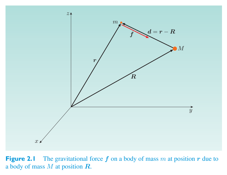
\(S'\), the position vectors and \(R'\) ≡ (\(X'\), \(Y'\), \(Z'\)) = (X − V t, Y, Z), but the displacement between the bodies will be \(d'\) = \(r'\) − \(R'\) = (x − X, y − Y, z − Z), which is identical to the displacement d in frame S. It follows that the magnitude of the displacement \(d'\) and the unit vector d \(E'\) in the direction of the displacement will also retain their old values. Since masses are invariant in Galilean relativity, we thus see that Newton’s law of universal gravitation takes the same form in S and \(S'\). Consequently, we can conclude that, at least in the case of gravitational forces, Newton’s second law of motion, f = m a, also takes the same form in frames S and \(S'\), and by implication in all inertial frames. All we have to do to find the form of the law in frame \(S'\) is to add primes to all the old quantities, remembering that in the case of invariants the primes will be irrelevant since the primed quantities will have the same values as the unprimed quantities.\(S'\),位置向量和 \(R'\) == (\(X'\), \(Y'\), \(Z'\)) = (X − V t, Y, Z),但物体之间的位移将为 \(d'\) = \(r'\) − \(R'\) = (x − X, y − Y, z − Z),这与坐标系 S 中的位移 d。 由此可见,位移 \(d'\) 的大小和位移方向上的单位向量 d \(E'\) 也将保留其旧值。由于质量在伽利略相对论中是不变的,因此我们看到牛顿万有引力定律在 S 和 \(S'\) 中具有相同的形式。因此,我们可以得出结论,至少在引力的情况下,牛顿第二运动定律 f = m a 在框架 S 和 \(S'\) 中也采取相同的形式,并且暗示在所有惯性系中。要在 \(S'\) 框架中找到定律的形式,我们所要做的就是将素数添加到所有旧量中,记住,在不变量的情况下,素数将是无关的,因为带素数的量将与未带素数的量具有相同的值。
An equation that is form-invariant under a given coordinate transformation is sometimes said to be covariant under that transformation. In the particular case that we have been considering, not only have we shown that Newton’s second law is covariant under the Galilean transformation, we have also concluded that the forces, masses and accelerations will have the same values in all inertial frames. So in this case, in addition to establishing the covariance of the equations, we have also shown the invariance of the quantities involved. Later in this chapter you will meet examples of physical laws that are covariant under a transformation but where the quantities involved are certainly not invariant.在给定坐标变换下形式不变的方程有时被称为在该变换下是协变的。在我们一直在考虑的特定情况下,我们不仅证明了牛顿第二定律在伽利略变换下是协变的,而且还得出了力、质量和加速度在所有惯性系中具有相同值的结论。因此,在这种情况下,除了建立方程的协方差之外,我们还证明了所涉及的量的不变性。在本章后面,您将遇到一些物理定律的示例,这些物理定律在变换下是协变的,但所涉及的数量肯定不是不变的。
The argument that we have already applied to Newton’s second law in the case of gravitational forces can be extended to any force that depends only on a combination of displacements and invariants. Such an extension would include Hooke’s law (for the force produced by the stretching of a spring) and even Coulomb’s law of electrostatic forces. However, the argument cannot be extended to all conceivable forces. It does not, for example, work for electromagnetic forces that depend on the velocity of a charged particle. Of course, this failure is not a great concern to us since we have already seen that it was problems arising from electromagnetism and light that persuaded Einstein to reject Galilean relativity in favour of special relativity, even at the price of having to accept new laws of mechanics.我们已经在引力情况下应用于牛顿第二定律的论点可以扩展到任何仅依赖于位移和不变量组合的力。这样的扩展将包括胡克定律(针对弹簧拉伸产生的力),甚至库仑静电力定律。然而,这一论点不能扩展到所有可以想象的力量。例如,它不适用于取决于带电粒子速度的电磁力。当然,这种失败并不是我们所关心的,因为我们已经看到,正是电磁学和光引起的问题说服了爱因斯坦拒绝伽利略相对论而支持狭义相对论,甚至不惜以接受新的力学定律为代价。
So, now that the idea of covariance or form-invariance has been introduced in the relatively simple context of Galilean relativity, let us return to special relativity and go in search of laws of mechanics that are covariant under the Lorentz transformations.因此,现在协变或形式不变的概念已经在伽利略相对论相对简单的背景下引入,让我们回到狭义相对论并寻找洛伦兹变换下协变的力学定律。
2.2 The laws of mechanics2.2 力学定律
2.2.1 Relativistic momentum2.2.1 相对论动量
The best place to start the reformulation of mechanics is with the concept of momentum. This quantity plays a crucial role in the analysis of high-speed collisions between fundamental particles, one of the main areas where relativistic mechanics (i.e. Lorentz-covariant mechanics) is routinely used. Relativistic mechanics will be essential to the analysis of the high-energy proton–proton collisions in the Large Hadron Collider (Figure 2.2 overleaf) at CERN, near Geneva.重新表述力学的最佳起点是动量概念。这个量在基本粒子之间的高速碰撞分析中起着至关重要的作用,这是相对论力学(即洛伦兹协变力学)常规使用的主要领域之一。相对论力学对于分析日内瓦附近欧洲核子研究中心大型强子对撞机(背页图 2.2)中的高能质子对撞机至关重要。
In Newtonian mechanics, the momentum of a particle of mass m travelling with velocity v is given by p Newtonian = m v. The importance of momentum comes mainly from the observation that, provided that no external forces act on a system,在牛顿力学中,质量为 m 以速度 v 运动的粒子的动量由 p Newtonian = m v 给出。动量的重要性主要来自于观察,假设没有外力作用在系统上,
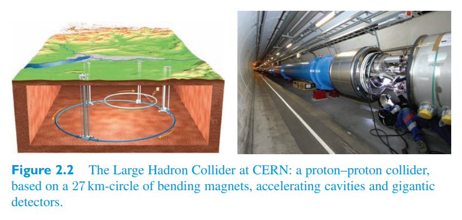
cavities and gigantic空洞和巨大的
This means, travelling with some travelling with initial v A and v B of those two这意味着,与一些以这两个的初始 v A 和 v B 一起旅行
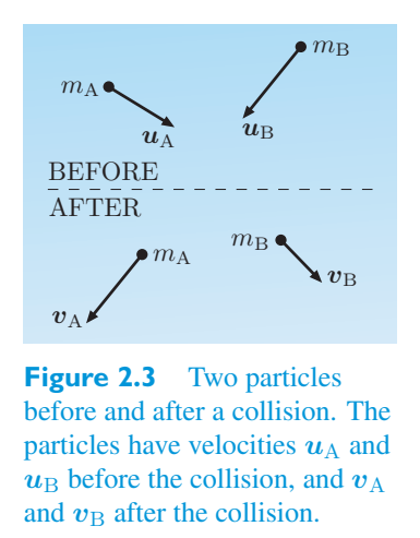
transforming velocities in the Newtonian way raises doubts about the Detailed calculations momentum is conserved shows that it cannot be should seek a new definition of momentum, sometimes called relativistic momentum, that will transform simply under Lorentz transformations and will provide a conservation law that is Lorentz-covariant. Of course, in formulating a new definition of momentum, we should not forget that physicists spent many years believing that experiments supported the conservation of Newtonian momentum — we should also aim to account for that.以牛顿方式变换速度引起了对动量守恒的详细计算的怀疑,表明不能寻求新的动量定义,有时称为相对论动量,它将在洛伦兹变换下简单地变换,并提供洛伦兹协变的守恒定律。当然,在制定动量的新定义时,我们不应忘记物理学家多年来相信实验支持牛顿动量守恒——我们也应该致力于解释这一点。
Consider a particle of mass m travelling with uniform velocity v between two (\(\Delta t\), \(\Delta x\), \(\Delta y\), \(\Delta z\)). events, labelled 1 and 2, separated by the coordinate intervals What makes the Newtonian momentum of such a particle transform in a complicated way is its direct relationship to the particle’s velocity:考虑质量为 m 的粒子以匀速 v 在两个粒子 (\(\Delta t\)、\(\Delta x\)、\(\Delta y\)、\(\Delta z\)) 之间移动。事件,标记为 1 和 2,由坐标间隔分隔。使此类粒子的牛顿动量以复杂方式变换的原因在于它与粒子速度的直接关系:
\(\Delta t\) transform in This involves ratios such as \(\Delta x\)/\(\Delta t\) where both \(\Delta x\) and moderately complicated ways. Momentum would transform far more simply if all references to the time between the two events, \(\Delta t\), were replaced by references to the proper time between the events, \(\Delta \tau\), which is an invariant and therefore transforms very simply. This suggests that a simple definition of the relativistic momentum of the particle would be\(\Delta t\) 变换这涉及诸如 \(\Delta x\)/\(\Delta t\) 之类的比率,其中 \(\Delta x\) 和中等复杂的方式。如果对两个事件之间的时间 \(\Delta t\) 的所有引用都替换为对事件之间的正确时间 \(\Delta \tau\) 的引用(\(\Delta \tau\) 是一个不变量,因此转换非常简单),那么动量的转换就会简单得多。这表明粒子相对论动量的简单定义是
Since the particle mass m and the proper time interval \(\Delta \tau\) are both invariants, relativistic momentum defined like this will transform in the same way as the displacement vector (\(\Delta x\), \(\Delta y\), \(\Delta z\)). Moreover, it follows from our discussion of proper time in Chapter 1 that since a particle travelling with speed v is present at both event 1 and event 2, the time between those events, \(\Delta t\), is related to the proper time between them by \(\Delta t =\)\(\gamma(v)\) \(\Delta \tau\), so we can rewrite the definition of relativistic momentum as由于粒子质量 m 和本征时间间隔 \(\Delta \tau\) 都是不变量,因此这样定义的相对论动量将以与位移矢量 (\(\Delta x\), \(\Delta y\), \(\Delta z\)) 相同的方式变换。此外,根据我们在第一章中对本征时间的讨论,由于事件 1 和事件 2 中都存在以速度 v 行进的粒子,因此这些事件之间的时间 \(\Delta t\) 与它们之间的本征时间相关,关系为 \(\Delta t =\)\(\gamma(v)\) \(\Delta \tau\),因此我们可以将相对论动量的定义重写为
We now have a clear definition of relativistic momentum that is guaranteed to transform simply between different inertial frames. However, several issues remain to be resolved before we can accept it. First, does it lead to a Lorentz-covariant conservation law, so that the observed conservation of momentum in one inertial frame implies the conservation of momentum in all inertial frames? Second, is such a conservation law correct: is momentum defined in this new way really conserved in any inertial frame? (Remember, covariance establishes the acceptability of a law in principle, but only experiment can establish its truth in practice.) Third, how does this newly defined relativistic momentum relate to Newtonian momentum? Let’s deal with the last of these questions first.我们现在对相对论动量有了一个明确的定义,保证它可以在不同的惯性系之间简单地转换。然而,在我们接受之前,还有几个问题需要解决。首先,它是否会导致洛伦兹协变守恒定律,因此在一个惯性系中观察到的动量守恒意味着所有惯性系中的动量守恒?其次,这样的守恒定律是否正确:以这种新方式定义的动量在任何惯性系中真的守恒吗? (请记住,协变原则上确立了定律的可接受性,但只有实验才能在实践中确立其真理。)第三,这种新定义的相对论动量与牛顿动量有何关系?让我们先解决最后一个问题。
The relativistic momentum p = mγ (v) v differs from Newtonian momentum only by a Lorentz factor \(\gamma(v)\). This means that at speeds that are small compared with the speed of light, where \(\gamma(v)\) ≈ 1, the two will be almost indistinguishable and all the apparent successes of Newtonian momentum conservation can be recovered.相对论动量 p = mγ (v) v 与牛顿动量的区别仅在于洛伦兹因子 \(\gamma(v)\)。这意味着,在与光速相比较小的速度下,其中 \(\gamma(v)\) ≈ 1,两者几乎无法区分,并且可以恢复牛顿动量守恒的所有明显成功。
As far as the covariance of relativistic momentum conservation is concerned, the question is this: if in some frame S就相对论动量守恒的协方差而言,问题是:如果在某个坐标系 S
will the velocity transformations also show that in some other inertial frame \(S'\)速度变换是否也表明在其他一些惯性系中 \(S'\)
Note that there are no primes on any of the masses in this last equation — that’s because they are invariant.请注意,最后一个方程中的任何质量上都没有素数 - 这是因为它们是不变的。
We could perform a detailed calculation to show that the law of relativistic momentum conservation is covariant under Lorentz transformations, but it’s really not necessary. There is a much neater way of reaching the same conclusion based on the fact that the relativistic momentum (\(p_{x}\), \(p_{y}\), \(p_{z}\)) transforms in the same way as the displacement vector (\(\Delta x\), \(\Delta y\), \(\Delta z\)). Suppose that we let the initial momenta in frame S be p A and p B, and let the final momenta be p A and p B. Then relativistic momentum conservation implies that p A + p B = p A + p B, or, after a slight rearrangement,我们可以通过详细的计算来证明相对论动量守恒定律在洛伦兹变换下是协变的,但这其实没有必要。基于相对论动量 (\(p_{x}\), \(p_{y}\), \(p_{z}\)) 以与位移矢量 (\(\Delta x\), \(\Delta y\), \(\Delta z\)) 相同的方式变换这一事实,有一种更简洁的方法可以得出相同的结论。假设我们令 S 系中的初始动量为 p A 和 p B,最终动量为 p A 和 p B。则相对论动量守恒意味着 p A + p B = p A + p B,或者稍微重新排列后,
Now, this equation can be represented geometrically as in Figure 2.4. With the arrows corresponding to the final momenta reversed in direction, the four arrows representing the individual momenta in frame S form a closed figure when drawn head to tail. Under a Lorentz transformation to some other frame, all of these momenta may change, but since they transform like displacement vectors, it will still be the case, even after transformation, that they will form a closed figure. Hence we can be sure that the transformed momenta will obey现在,这个方程可以用几何表示,如图 2.4 所示。由于最终动量对应的箭头方向相反,S 系中代表各个动量的四个箭头从头到尾绘制时形成一个闭合图形。在洛伦兹变换到其他坐标系下,所有这些动量都可能发生变化,但由于它们像位移矢量一样变换,因此即使在变换之后,它们仍然会形成一个闭合图形。因此我们可以确定变换后的动量将服从
and consequently \(p'_{A}\) + \(p'_{B}\) = \(p'_{A}\) + \(p'_{B}\). Thus we see, in this case at least, that if relativistic momentum is conserved in one inertial frame, then it will be conserved in all inertial frames. This geometric argument can be extended to as many colliding particles as we want, so the argument shows that relativistic momentum conservation is a Lorentz-covariant result.因此,\(p'_{A}\) + \(p'_{B}\) = \(p'_{A}\) + \(p'_{B}\)。因此,至少在这种情况下,我们看到,如果相对论动量在一个惯性系中守恒,那么它在所有惯性系中也将守恒。这个几何论证可以扩展到我们想要的任意数量的碰撞粒子,因此该论证表明相对论动量守恒是洛伦兹协变的结果。
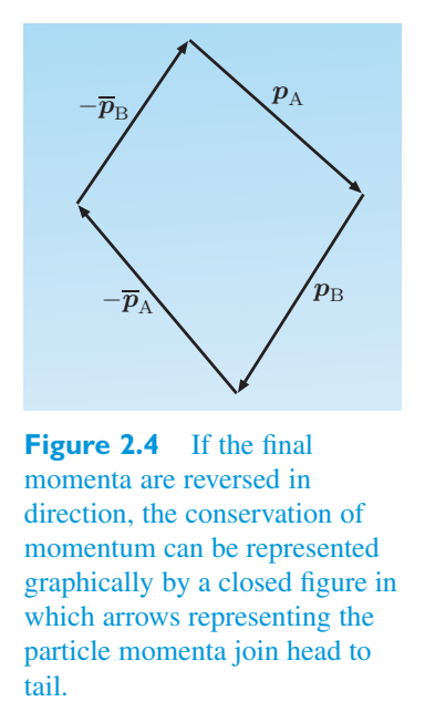
- ● Why can’t this same geometric argument be used to● 为什么不能使用相同的几何参数
show that Newtonian momentum, if conserved in some inertial frame S, will also be conserved in all other inertial frames, even under Lorentz transformations?表明牛顿动量如果在某些惯性系 S 中守恒,那么即使在洛伦兹变换下,在所有其他惯性系中也将守恒?
❍ This is because Newtonian momentum does not transform in the same way as a displacement vector under a Lorentz transformation. Even if the Newtonian momentum vectors formed a closed figure in frame S, the complicated transformation law of Newtonian momentum would ensure that they did not form a closed figure in all other inertial frames.❍ 这是因为牛顿动量在洛伦兹变换下的变换方式与位移矢量不同。即使牛顿动量矢量在S系中形成闭图形,牛顿动量复杂的变换规律也将确保它们在所有其他惯性系中不会形成闭图形。
Now the only remaining question is: ‘does nature really make use of this possibility?’ Here experiment is the arbiter, and the analysis of an enormous number of high-speed particle collisions clearly indicates that nature does so. It is relativistic momentum that is found to be conserved in nature. So we can conclude the following.现在唯一剩下的问题是:“大自然真的利用了这种可能性吗?”这里实验是仲裁者,对大量高速粒子碰撞的分析清楚地表明大自然确实这样做了。人们发现,相对论动量在自然界中是守恒的。所以我们可以得出以下结论。
Relativistic momentum相对论动量
In Lorentz-covariant mechanics, the relativistic momentum of a particle of mass m moving with velocity v is defined as在洛伦兹协变力学中,质量为 m 以速度 v 运动的粒子的相对论动量定义为
The total relativistic momentum of a system is conserved in the absence of external forces.在没有外力的情况下,系统的总相对论动量是守恒的。
Exercise 2.1 An electron of mass m = 9.11 × 10 −练习 2.1 质量为 m = 9.11 × 10 − 的电子
31 kg has speed 4 c/5. What is the magnitude of its (relativistic) momentum?31公斤的速度为4 c/5。它的(相对论)动量有多大?
2.2.2 Relativistic kinetic energy2.2.2 相对论动能
Another quantity of importance in mechanics is kinetic energy. As in the case of momentum, special relativity demands that we modify the definition of kinetic energy before it can take its proper place in a Lorentz-covariant formulation of mechanics.力学中另一个重要的量是动能。与动量的情况一样,狭义相对论要求我们修改动能的定义,然后才能在力学的洛伦兹协变公式中占据适当的位置。
In Newtonian mechanics, the kinetic energy of a particle travelling with speed v can be found from the work W done in accelerating that particle from rest to its final speed v. If we consider the case of a particle with speed u accelerated along the x -axis by a force of magnitude f, we can write the kinetic energy as在牛顿力学中,以速度 v 行进的粒子的动能可以通过将该粒子从静止加速到最终速度 v 所做的功 W 求得。如果我们考虑速度为 u 的粒子被大小为 f 的力沿 x 轴加速的情况,我们可以将动能写为
In Newtonian mechanics, the applied force is the same as the rate of change of momentum, f = ma = m d v/d t = d p/d t, so在牛顿力学中,施加的力与动量的变化率相同,f = ma = m d v/d t = d p/d t,因此
The integral can be rewritten in a much more useful form by changing integration variables and using the chain rule:通过更改积分变量并使用链式法则,可以将积分重写为更有用的形式:
In this way a Newtonian expression for kinetic energy that initially involved distance and force can be re-expressed in terms of speed u and momentum magnitude p. This latter expression can be taken over to special relativity, where we already know the relationship between speed and the magnitude of momentum.这样,最初涉及距离和力的牛顿动能表达式可以用速度 u 和动量大小 p 重新表达。后一种表达可以采用狭义相对论,我们已经知道速度和动量大小之间的关系。
So, in special relativity, a reasonable starting point from which to define the relativistic kinetic energy of a particle of mass m moving with speed v is因此,在狭义相对论中,定义质量为 m、速度为 v 的粒子的相对论动能的合理起点是
This integral can be evaluated using the technique of integration by parts:该积分可以使用分部积分技术来计算:
The remaining integral can be performed by inspection, giving剩余积分可以通过检查进行,给出
A compact final result can be found by putting both terms over a common denominator:通过将两项放在一个公分母上可以找到紧凑的最终结果:
Thus the suggested expression for the relativistic kinetic energy of a particle of mass m moving with speed v is因此,质量为 m 以速度 v 运动的粒子的相对论动能的建议表达式为
There is no general principle of conservation of kinetic energy for us to consider in this case, but in Newtonian physics, kinetic energy is conserved in elastic collisions. In an elastic collision, the particles do not change their number, state or nature, so what goes in is also what comes out. As far as covariance under在这种情况下,我们没有考虑动能守恒的一般原理,但在牛顿物理学中,弹性碰撞中动能守恒。在弹性碰撞中,粒子的数量、状态或性质不会改变,所以进去的也是出来的。就协方差而言
Lorentz transformations is concerned, it is possible to show that in the case of elastic collisions, the proposed expression for relativistic kinetic energy does ensure that an elastic collision in one inertial frame will also be elastic in all other inertial frames.就洛伦兹变换而言,可以证明,在弹性碰撞的情况下,所提出的相对论动能表达式确实确保了一个惯性系中的弹性碰撞在所有其他惯性系中也将是弹性的。
How does the relativistic kinetic energy relate to the Newtonian kinetic energy? At first sight the relationship is not at all obvious, but it soon becomes clear if we factor, \(\gamma(v)\), obtained use the following mathematical expansion of the Lorentz via Taylor’s theorem or the binomial expansion:相对论动能与牛顿动能有何关系?乍一看,这种关系并不明显,但如果我们通过泰勒定理或二项式展开使用洛伦兹的以下数学展开式对 \(\gamma(v)\) 进行因式分解,很快就会变得清晰:
The expansion continues with higher orders of \(v^{2}\)/\(c^2\). In Newtonian physics, the speed v will generally be small compared with the speed of light c, so these expression for \(\gamma(v)\) higher-order terms can be ignored. Substituting the truncated into Equation 2.19 gives随着 \(v^{2}\)/\(c^2\) 订单的增加,扩展仍在继续。在牛顿物理学中,速度 v 与光速 c 相比通常会很小,因此 \(\gamma(v)\) 高阶项的这些表达式可以忽略。将截断代入公式 2.19 得出
So the Newtonian expression for kinetic energy emerges as a low-speed approximation to the relativistic expression. All the low-speed experiments that support the Newtonian expression will also support the more general expression of relativistic mechanics.因此,牛顿动能表达式是相对论表达式的低速近似。所有支持牛顿表达式的低速实验也将支持相对论力学的更一般的表达式。
Henceforth we shall adopt the proposed definition, so we can say the following.今后我们将采用提议的定义,因此我们可以说以下内容。
Relativistic kinetic energy相对论动能
In Lorentz-covariant mechanics, the relativistic kinetic energy of a particle of mass m moving with speed v is在洛伦兹协变力学中,质量为 m 以速度 v 运动的粒子的相对论动能为
Exercise 2.2 Compute the kinetic energy of a muon练习2.2 计算\(\mu\)子的动能
(mass m = \(1.88\times10^{-28}\) kg) travelling with speed 9 c/10.(质量 m = \(1.88\times10^{-28}\) kg)以 9 c/10 的速度行驶。
2.2.3 Total relativistic energy and mass2.2.3 总相对论能量和质量
energy活力
In the 1905 paper in which Einstein introduced the special theory of relativity, he considered the acceleration of an electron and arrived at the expressions for momentum and kinetic energy that have been introduced in this chapter. However, our next topic is one that was not considered in that first paper. It concerns the best known result of special relativity, E = \(mc^2\), and the ‘equivalence’ between mass and energy that it is usually said to indicate. It was first indicated in a three-page paper (‘Does the inertia of a body depend upon its energy content?’) published a few months after the first paper, and then more fully developed in later publications.在 1905 年爱因斯坦介绍狭义相对论的论文中,他考虑了电子的加速,并得出了本章介绍的动量和动能的表达式。然而,我们的下一个主题是第一篇论文中未考虑的主题。它涉及狭义相对论最著名的结果 E = \(mc^2\),以及通常所说的质量和能量之间的“等价性”。它首先在一篇三页纸的论文(“物体的惯性取决于其能量含量吗?”)中指出,该论文在第一篇论文发表几个月后发表,然后在后来的出版物中得到了更充分的发展。
The crucial result is already suggested by the expression for relativistic kinetic energy E = (\(\gamma(v)\) − 1) \(mc^2\), which can be rewritten as相对论动能 E = (\(\gamma(v)\) − 1) \(mc^2\) 的表达式已经表明了关键结果,该表达式可以重写为
This is now interpreted as showing that in an inertial frame S, where a particle of mass m has speed v, that particle will have a total relativistic energy E = \(\gamma(v)\) \(mc^2\) that is the sum of a relativistic kinetic energy \(E_K\) and a mass energy \(E_0\) = \(mc^2\). As a mere rearrangement and renaming of terms, this is a harmless exercise. The revolutionary step is in the proposal that in relativistic mechanics generally, and high-speed particle collisions in particular, it is the total relativistic energy that is conserved. In high-speed collisions, neither kinetic energy nor mass energy will necessarily be conserved, but their sum, represented by the total relativistic energy E, will be.现在这被解释为表明,在惯性系 S 中,质量为 m 的粒子具有速度 v,该粒子将具有总相对论能量 E = γ (v) mc 2,即相对论动能 \(E_K\) 和质量能量 \(E_0\) = mc 2 之和。作为仅仅是术语的重新排列和重命名,这是一种无害的练习。革命性的一步是提出,在一般的相对论力学中,特别是在高速粒子碰撞中,总的相对论能量是守恒的。在高速碰撞中,动能和质能都不一定守恒,但它们的总和(以相对论总能量 E 表示)将会守恒。
The startling possibility opened up by this suggestion is that in high-speed collisions, particles with mass may be created at the expense of relativistic kinetic energy. It is also possible for some or all of the particles involved in a collision to be annihilated, releasing mass energy that may emerge from the collision either as the mass energy of particles created in the collision or as a contribution to the kinetic energy of all the particles that emerge, or both. This takes relativistic mechanics into an important domain that was completely unexplored by Newtonian mechanics.这一建议所揭示的令人震惊的可能性是,在高速碰撞中,具有质量的粒子可能会以相对论动能为代价而产生。参与碰撞的部分或全部粒子也有可能被湮灭,释放出碰撞中产生的质量能,或者作为碰撞中产生的粒子的质量能,或者作为对所有出现的粒子的动能的贡献,或者两者兼而有之。这将相对论力学带入了牛顿力学完全未探索过的重要领域。
It’s worth noting that the relationship between mass and energy represented by the formula \(E_0\) = \(mc^2\) is not limited to high-speed particle collisions. The initial arguments in favour of such a relationship were based on considerations of the emission of radiation from a body, and it has often been stressed that in the case of a composite body, such as a piece of metal, the simple act of heating it so as to raise its temperature will increase its internal energy and thereby increase its mass. Note that this has nothing to do with the speed of the body; it is a change in the invariant mass that we are discussing.值得注意的是,\(E_0\) = mc 2 公式所表示的质量与能量的关系并不局限于高速粒子碰撞。支持这种关系的最初论据是基于对物体辐射发射的考虑,并且经常强调,在复合物体(例如一块金属)的情况下,加热它以提高其温度的简单行为将增加其内能,从而增加其质量。请注意,这与身体的速度无关;我们正在讨论的是不变质量的变化。
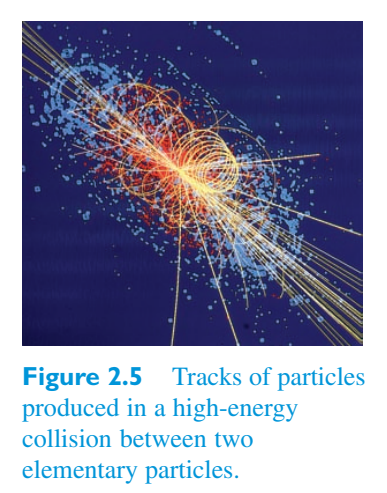
When Einstein first proposed the equivalence of mass and energy, he suggested that it might account for the energy associated with radioactive decay. This is now known to be the case. \(E_0\) = \(mc^2\) plays a vital role in explaining many nuclear phenomena, and particle creation (see Figure 2.5) is the basis of much of the work carried out in particle physics laboratories. Ironically, Einstein’s famous relation has also become indissolubly linked with the awesome energy release of nuclear weapons (Figure 2.6) despite Einstein’s many pronouncements on the need for world peace.当爱因斯坦首次提出质量和能量的等价性时,他认为这可以解释与放射性衰变相关的能量。现在已知情况确实如此。 \(E_0\) = mc 2 在解释许多核现象中起着至关重要的作用,而粒子的产生(见图 2.5)是粒子物理实验室中进行的许多工作的基础。具有讽刺意味的是,尽管爱因斯坦多次宣称需要世界和平,但爱因斯坦著名的关系也与核武器释放的惊人能量有着不可分割的联系(图2.6)。
Total relativistic energy and mass energy总相对论能量和质量能量
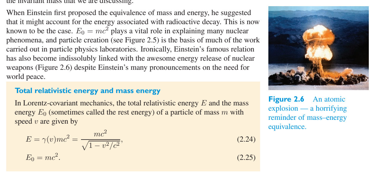
In Lorentz-covariant mechanics, the total relativistic energy E and the mass energy 0 (sometimes called the rest energy) of a particle of mass with speed are given by在洛伦兹协变力学中,具有速度的质量粒子的总相对论能量 E 和质量能量 0(有时称为静止能量)由下式给出
Exercise 2.3 The proton has mass m = 1.67 × 10练习 2.3 质子的质量 m = 1.67 × 10
− 27 kg. Compute the total 3 c/5. (relativistic) energy of a proton moving with speed v =- 27 公斤。计算总计 3 c/5。以速度 v 运动的质子的(相对论)能量 =
Exercise 2.4 At what speed is the total energy of a练习2.4 物体速度为多少时,其总能量为
particle twice the mass energy?粒子质量能量的两倍?
Exercise 2.5 (a) In a nuclear fission of uranium- 235练习2.5(a)在铀的核裂变中- 235
caused by the absorption of a neutron, nuclei of krypton and barium are produced, and three neutrons are emitted. The difference in the total mass of the particles present at the start of the process and those present at the end is \(3.08\times10^{-28}\) kg. What is the energy (1 eV = \(1.60\times10^{-19}\) J)? released in this process, in both joules and electronvolts由于吸收一个中子,产生氪和钡的原子核,并发射三个中子。过程开始时和结束时存在的颗粒总质量之差为 \(3.08\times10^{-28}\) kg。能量是多少(1 eV = \(1.60\times10^{-19}\) J)?在此过程中释放的能量,单位为焦耳和电子伏特
(b) Given that the binding energy of a hydrogen atom is 13.6 eV, what is the difference between the mass of a hydrogen atom and the masses of its constituent electron and proton?(b) 假设氢原子的结合能为 13.6 eV,氢原子的质量与其组成电子和质子的质量有什么区别?
2.2.4 Four-momentum2.2.4 四动量
In Chapter 1 you were briefly introduced to the four-position, that is, the four-component object在第一章中,您简要介绍了四位置,即四分量对象
which usefully combined space and time coordinates while using ct rather than t to ensure that they could all be expressed in units of distance. Often when writing \([x^{\mu}]\), it is convenient to write r instead of the three space components x, y and z, so we can write它有效地结合了空间和时间坐标,同时使用 ct 而不是 t 以确保它们都可以用距离单位表示。通常在写\([x^{\mu}]\)时,写r代替三个空间分量x、y和z会更方便,所以我们可以写
Now suppose that the four-position \([x^{\mu}]\) describes the events on the spacetime pathway (i.e. the world-line) of a particle of mass m. We can imagine that the particle carries a clock with it that records the proper time \(\tau\) between successive events as it moves along its world-line. We can then regard each component x \(\mu\) of the particle’s four-position \([x^{\mu}]\) as a function of proper time \(\tau\). Differentiating each of those components x \(\mu\) with respect to \(\tau\) gives us four so-called proper derivatives d x \(\mu\)/d \(\tau\) that we can use as the components of another four-component entity that we shall denote \([U^{\mu}]\). Thus现在假设四位 \([x^{\mu}]\) 描述了质量为 m 的粒子的时空路径(即世界线)上的事件。我们可以想象粒子携带一个时钟,记录它沿着其世界线移动时连续事件之间的固有时间 \(\tau\)。然后,我们可以将粒子四位置 \([x^{\mu}]\) 的每个分量 x \(\mu\) 视为本征时间 \(\tau\) 的函数。将每个分量 x \(\mu\) 相对于 \(\tau\) 求导,得到四个所谓的真导数 d x \(\mu\)/d \(\tau\),我们可以将其用作另一个四分量实体的分量,我们将其表示为 \([U^{\mu}]\)。因此
The derivatives d x/d \(\tau\), d y/d \(\tau\) and d z/d \(\tau\) that appear on the right can be regarded \(\Delta z\)/\(\Delta \tau\) that we as infinitesimal limits of the ratios \(\Delta x\)/\(\Delta \tau\), \(\Delta y\)/\(\Delta \tau\) and considered earlier when introducing relativistic momentum. On that earlier occasion, the relation \(\Delta t =\)\(\gamma(v)\) \(\Delta \tau\) was used to relate those ratios to the scaled velocity components \(\gamma(v)\) v, \(\gamma(v)\) v and \(\gamma(v)\) v. Doing the same here, and also noting that d t/d \(\tau\) is the limit of \(\Delta t\)/\(\Delta \tau =\)\(\gamma(v)\), we can write右侧出现的导数 d x/d \(\tau\)、d y/d \(\tau\) 和 d z/d \(\tau\) 可以视为 \(\Delta z\)/\(\Delta \tau\),我们将其视为比率 \(\Delta x\)/\(\Delta \tau\)、\(\Delta y\)/\(\Delta \tau\) 的无穷小极限,并在前面介绍时考虑过相对论动量。在那之前的情况下,关系 \(\Delta t =\)\(\gamma(v)\) \(\Delta \tau\) 用于将这些比率与缩放速度分量 \(\gamma(v)\) v、\(\gamma(v)\) v 和 \(\gamma(v)\) v 联系起来。在这里做同样的事情,并且还注意到 d t/d \(\tau\) 是\(\Delta t\)/\(\Delta \tau =\)\(\gamma(v)\),我们可以写
Since \([U^{\mu}]\) is the This quantity is called the four-velocity of the particle. \([U^{\mu}]\) behaves derivative of \([x^{\mu}]\) with respect to the invariant \(\tau\), the four-velocity just as the four-position does under Lorentz transformations.由于 \([U^{\mu}]\) 是该量称为粒子的四速度。 \([U^{\mu}]\) 表现为 \([x^{\mu}]\) 相对于不变 \(\tau\) 的导数,四速度就像洛伦兹变换下的四位置一样。
The four-velocity has an interesting property that becomes apparent when \([U^{\mu}]\) is combined with the Minkowski metric [\(\eta\) \(\mu\)\(\nu\)] that, was introduced in Chapter 1. In \(\eta\) \(\Delta x\) \(\mu\) \(\Delta x\) \(\nu\). Now we that earlier case, we met the invariant (\(\Delta s\)) 2 = 3 can see that四速度有一个有趣的属性,当 \([U^{\mu}]\) 与第 1 章中介绍的闵可夫斯基度规 [\(\eta\) \(\mu\)\(\nu\)] 相结合时,这个属性就变得很明显。现在我们在前面的情况下,遇到了不变式 (\(\Delta s\)) 2 = 3 可以看到
But since但自从
it is clear that the original sum has the invariant value显然原和具有不变值
Multiplying the four-velocity \([U^{\mu}]\) by the invariant mass m gives a related four-component entity called the four-momentum:将四速度 \([U^{\mu}]\) 乘以不变质量 m 得到一个相关的四分量实体,称为四动量:
All the terms on the right should already be familiar. The first is the total relativistic energy divided by the speed of light, E/c; the other three are the components of the relativistic momentum p, so we can write右边的所有术语应该已经很熟悉了。第一个是总相对论能量除以光速,E/c;另外三个是相对论动量 p 的分量,所以我们可以写成
It is clear that the four-momentum contains all the information about the relativistic energy and relativistic momentum of any particle.显然,四动量包含了任何粒子的相对论能量和相对论动量的所有信息。
The crucial point about all this is that under a Lorentz transformation from one inertial frame to another (S to \(S'\), say), the four-momentum \([P^{\mu}]\) transforms in exactly the same way as the four-position.所有这一切的关键点是,在从一个惯性系到另一个惯性系(例如 S 到 \(S'\))的洛伦兹变换下,四动量 \([P^{\mu}]\) 的变换方式与四位置完全相同。
- ● Why must the four-momentum transform in the same way as the为什么四动量必须以与四动量相同的方式转变?
four-position? ❍ Because \(\tau\) is an invariant, the four-velocity \([U^{\mu}]\) = \(\left[\frac{dx^\mu}{d\tau}\right]\) will transform in the same way as the four-position \([x^{\mu}]\). Since m is also invariant, it follows that the four-momentum \([P^{\mu}]\) = \([mU^{\mu}]\) must also transform like \([x^{\mu}]\).四位? ❍ 因为 \(\tau\) 是不变量,所以四速度 \([U^{\mu}]\) = \(\left[\frac{dx^\mu}{d\tau}\right]\) 将以与四位置 \([x^{\mu}]\) 相同的方式进行变换。由于 m 也是不变的,因此四动量 \([P^{\mu}]\) = \([mU^{\mu}]\) 也必须像 \([x^{\mu}]\) 一样变换。
As a result of the simple behaviour of \([P^{\mu}]\) under a Lorentz transformation, we can say that if the frames S and \(S'\) are in standard configuration, then a particle of mass m with velocity v, that has relativistic energy E and relativistic momentum p in inertial frame S, will be found to have energy \(E'\) and由于 \([P^{\mu}]\) 在洛伦兹变换下的简单行为,我们可以说,如果框架 S 和 \(S'\) 处于标准配置,则质量为 m 且速度为 v 的粒子,在惯性系 S 中具有相对论能量 E 和相对论动量 p,将发现具有能量 \(E'\) 和
Note that the particle speeds v and \(v'\) that help to determine the energy and momentum in S and \(S'\) are quite distinct from V, which represents the speed of frame \(S'\) as measured in frame S. For a particle travelling along the x -axis, so that v = (v, 0, 0), the relation between v, \(v'\) and V follows from the velocity V)/(1 − vV/\(c^2\)). transformation of Chapter 1, and is given by \(v'\) = (v −请注意,有助于确定 S 和 \(S'\) 中的能量和动量的粒子速度 v 和 \(v'\) 与 V 完全不同,V 代表在坐标系 S 中测量的坐标系 \(S'\) 的速度。对于沿 x 轴运动的粒子,使得 v = (v, 0, 0),v、\(v'\) 和 V 之间的关系由速度 V)/(1 − vV/\(c^2\))。第 1 章的变换,由下式给出: \(v'\) = (v −
As was the case with the four-position, the transformation rule for four-momentum can be written in a number of equivalent ways using the Lorentz transformation matrix [\(\Lambda\) \(\mu\) \(\nu\)]. In terms of matrices,与四位置的情况一样,四动量的变换规则可以使用洛伦兹变换矩阵 [\(\Lambda\) \(\mu\) \(\nu\)] 以多种等效方式编写。就矩阵而言,
which may be represented more compactly as可以更紧凑地表示为
Alternatively, we can represent the transformation using components and summations:或者,我们可以使用分量和求和来表示变换:
The fact that the four-momentum transforms in exactly the same way as the four-position says something quite profound about energy and momentum. Under Lorentz transformation, the energy and momentum components intertwine, and can be thought of as aspects of a single quantity, just as space and time are unified into spacetime. That which is energy to one observer is a mix of energy and momentum to another.事实上,四动量的变换方式与四位置的变换方式完全相同,这一事实说明了有关能量和动量的深刻含义。在洛伦兹变换下,能量和动量分量交织在一起,可以被视为单个量的各个方面,就像空间和时间统一为时空一样。对于一个观察者来说是能量,对于另一个观察者来说则是能量和动量的混合体。
Exercise 2.6 In frame of reference S, an √ electron moving练习 2.6 在参考系 S 中,一个 √ 电子移动
along the x -axis has energy 3 m e \(c^2\) and momentum magnitude 8 m e c. Use the transformations of energy and momentum to find the energy and momentum magnitude observed in x -direction. frame \(S'\) moving with speed 4 c/5 relative to S in the positive沿 x 轴的能量为 3 m e \(c^2\),动量大小为 8 m e c。使用能量和动量的变换来查找在 x 方向上观察到的能量和动量大小。坐标系 \(S'\) 相对于 S 正向以 4 c/5 的速度移动
2.2.5 The energy–momentum relation2.2.5 能量-动量关系
It was shown in Equation 2.31 that公式 2.31 表明
Since \([P^{\mu}]\) is defined by \([P^{\mu}]\) = m \([U^{\mu}]\), it follows that由于 \([P^{\mu}]\) 由 \([P^{\mu}]\) = m \([U^{\mu}]\) 定义,因此
But using the Minkowski metric we also know that但使用闵可夫斯基度规我们也知道
Consequently, we can say that因此,我们可以说
So, regardless of the frame of reference of an observer, the difference between the squared total energy and the squared momentum magnitude multiplied by the speed of light squared is proportional to the squared invariant mass. This extremely useful relationship is often called the energy–momentum relation and is usually written as follows.因此,无论观察者的参考系如何,总能量平方与动量大小平方乘以光速平方之间的差值与不变质量平方成正比。这种非常有用的关系通常称为能量-动量关系,通常写如下。
Energy–momentum relation能量-动量关系
Taking the positive square root, we see that取正平方根,我们看到
A plot of this relation can be seen in Figure 2.7. Apart from the presence of the distinctly non-Newtonian rest energy \(E_0\) = \(mc^2\), the behaviour at low speeds (when p is close to zero) is what would be expected in Newtonian mechanics, with (kinetic) energy increasing in proportion to \(p^{2}\). However, as the momentum magnitude increases, the total energy becomes more and more nearly proportional to the momentum magnitude, as special relativity requires.这种关系的图如图 2.7 所示。除了存在明显的非牛顿静止能量 \(E_0\) = mc 2 之外,低速时的行为(当 p 接近于零时)也是牛顿力学所期望的,(动能)能量与 p 2 成比例增加。然而,随着动量大小的增加,总能量变得越来越接近与动量大小成正比,正如狭义相对论所要求的那样。
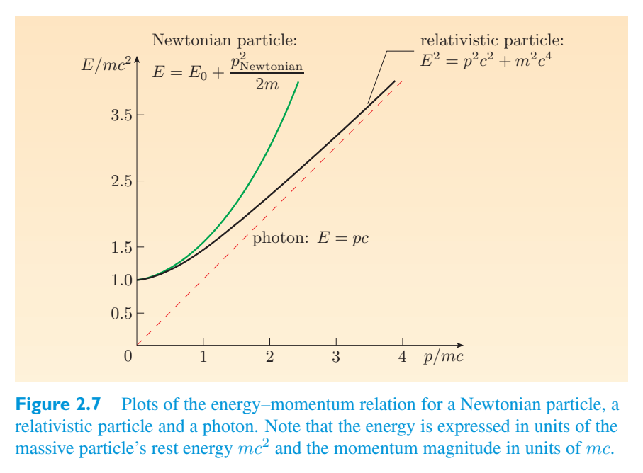
- ● The electron has mass m e = \(9.11\times10^{-31}\) kg. What is the energy of an电子的质量为 m e = \(9.11\times10^{-31}\) kg。一个物体的能量是多少
electron that has a momentum of magnitude \(1.00\times10^{-22}\) \(\mathrm{kg\,m\,s^{-1}}\)? ❍ Making the substitutions \(m^{2}\) \(c^4\) = \(6.72\times10^{-27}\) J and \(c^2\) \(p^{2}\) = \(9.00\times10^{-28}\) J, the energy–momentum √ relation shows that the energy is E = \(6.72\times10^{-27}\) + \(9.00\times10^{-28}\) J = \(8.73\times10^{-14}\) J.动量大小为 \(1.00\times10^{-22}\) \(\mathrm{kg\,m\,s^{-1}}\) 的电子? ❍ 将 m 2 \(c^4\) = \(6.72\times10^{-27}\) J 和 \(c^2\) p 2 = \(9.00\times10^{-28}\) J 代入,则能量-动量 √ 关系表明,能量为 E = \(6.72\times10^{-27}\) + \(9.00\times10^{-28}\) J = \(8.73\times10^{-14}\) J。
The energy–momentum relation has an important consequence with no analogue in Newtonian mechanics. A symmetry principle known as gauge-invariance, which is of great importance in particle physics, demands that the photon, which is often described as the ‘particle of light’, should be strictly massless with m = 0. It follows from the energy–momentum relation that for a photon, or any other massless particle,能量-动量关系具有牛顿力学中无可比拟的重要结论。被称为规范不变性的对称原理在粒子物理学中非常重要,它要求通常被描述为“光粒子”的光子应该严格无质量,m = 0。从能量-动量关系可以得出,对于光子或任何其他无质量粒子,
The photon carries energy, so even though it has no mass, it does have a momentum. This clearly shows the non-Newtonian nature of relativistic momentum.光子携带能量,因此即使它没有质量,它也有动量。这清楚地表明了相对论动量的非牛顿性质。
It has been suggested that the momentum of the photon could be harnessed to make solar sails, a kind of propulsion system for spacecraft. A depiction of a solar-sail craft is shown in Figure 2.8.有人建议可以利用光子的动量来制造太阳帆,一种航天器的推进系统。太阳帆飞船的描述如图 2.8 所示。
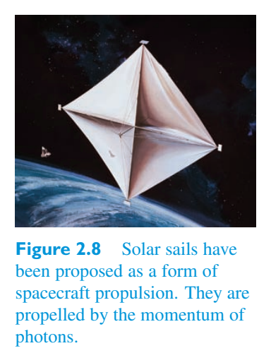
h = \(6.63\times10^{-34}\) \(\mathrm{J\,s}\) ish = \(6.63\times10^{-34}\) \(\mathrm{J\,s}\) 是
Exercise 2.7 (a) The energy of a photon is hf, where练习2.7 (a) 光子的能量是hf,其中
Planck’s constant and f is the frequency of the photon. What is the magnitude of the momentum of a single photon belonging to a monochromatic beam of light with frequency \(5.00\times10^{14}\) Hz?普朗克常数,f 是光子的频率。属于频率为 \(5.00\times10^{14}\) Hz 的单色光束的单个光子的动量大小是多少?
(b) At what rate must such photons be absorbed by a solar sail if they are to cause a steady force of magnitude 10 N on the sail?(b) 如果这些光子要在太阳帆上产生 10 N 量级的稳定力,那么它们必须以什么速率被太阳帆吸收?
Exercise 2.8 You are told by a scientist of ill repute练习 2.8 一位声名狼藉的科学家告诉你
that a ficteron particle of mass m f has been measured to have energy E f = 3 m f \(c^2\) and momentum of magnitude p f = 7 m f c. Are those values consistent with special relativity?质量为 m f 的菲克特粒子已被测量为具有能量 E f = 3 m f \(c^2\) 和动量大小 p f = 7 m f c。这些值符合狭义相对论吗?
2.2.6 The conservation of energy and momentum2.2.6 能量和动量守恒
Now that we know how the four-momentum transforms under a Lorentz transformation, it is easy to demonstrate the Lorentz covariance of the conservation laws of relativistic energy and momentum.现在我们知道了四动量在洛伦兹变换下是如何变换的,就很容易证明相对论能量和动量守恒定律的洛伦兹协变性了。
particles emerge. Let Imagine a collision in which N particles collide, and N incident particle i have mass m i and an incident four-momentum (i = 1, 2, 3,..., N), and remember that some of the masses may be zero. Similarly, let the particles that emerge from the collision have masses m j and four-momenta \([P^{\nu}]\) (j = 1, 2, 3,..., N). Note that the index representing the particle has been placed in parentheses to avoid confusing it with the index that denotes a particular component of the four-momentum. The conservation of energy and momentum in an inertial frame S is represented by the relation粒子出现。想象一次碰撞,其中 N 个粒子发生碰撞,N 个入射粒子 i 具有质量 m i 和入射四动量 (i = 1, 2, 3,..., N),并记住某些质量可能为零。类似地,让碰撞中出现的粒子具有质量 m j 和四动量 \([P^{\nu}]\) (j = 1, 2, 3,..., N)。请注意,代表粒子的索引已放在括号中,以避免将其与表示四动量特定分量的索引混淆。惯性系 S 中的能量和动量守恒由以下关系表示
Note that \(\nu\) is a free index in this expression, so this one line really represents four different equations, one for each possible value of \(\nu\).请注意,\(\nu\) 在此表达式中是一个自由索引,因此这一行实际上代表四个不同的方程,每个方程对应 \(\nu\) 的每个可能值。
What will be the energy and momentum involved in this collision as observed by some other inertial observer who uses frame \(S'\)? Performing the same Lorentz transformation on each side of the equation, we see that使用 \(S'\) 系的其他惯性观察者观察到的这次碰撞涉及的能量和动量是多少?在方程的每一边执行相同的洛伦兹变换,我们看到
Since the transformation law of an individual four-momentum takes the form [\(P'\) \(\mu\)] = [\(\Lambda\) \(\mu\)] \([P^{\nu}]\), we know that each individual four-momentum in the sum will transform in the same way under the Lorentz transformation to frame \(S'\). Consequently, transforming both sides of the conservation law, we get由于单个四动量的变换定律采用 [\(P'\) \(\mu\)] = [\(\Lambda\) \(\mu\)] \([P^{\nu}]\) 的形式,我们知道在洛伦兹变换下,总和中的每个单独的四动量将以相同的方式变换到坐标系 \(S'\)。因此,变换守恒定律两边,我们得到
Apart from an irrelevant switch in the symbol used to represent the free index, from \(\nu\) to \(\mu\), the only difference between the conservation law in frame S and that in frame \(S'\) is the addition of some primes.除了用于表示自由索引的符号中不相关的转换(从 \(\nu\) 到 \(\mu\))之外,框架 S 中的守恒定律与框架 \(S'\) 中的守恒定律之间的唯一区别是添加了一些素数。
The lesson is clear: by expressing the conservation laws of relativistic energy and relativistic momentum in terms of four-momenta that transform simply under Lorentz transformations, it has become obvious that the conservation laws can be written in the same form in all inertial frames without any need to carry out complicated transformations of E and p. In such situations we say that the law is manifestly covariant. This is only a first glimpse of manifest covariance. We shall have much more to say on the subject later.教训很清楚:通过用洛伦兹变换下简单变换的四动量来表达相对论能量和相对论动量守恒定律,很明显,守恒定律可以在所有惯性系中以相同的形式写出,而不需要对 E 和 p 进行复杂的变换。在这种情况下,我们说该定律是明显协变的。这只是显性协方差的初步体现。稍后我们将就这个主题有更多的内容要说。
2.2.7 Four-force2.2.7 四力
The last major mechanics concept that we shall discuss is that of force. Recalling that in Newtonian particle mechanics, force may be defined by the rate of change of momentum, and taking the introduction of the four-velocity as a guide, a natural way to introduce a four-force in relativistic mechanics is via the manifestly covariant relation我们要讨论的最后一个主要力学概念是力的概念。回想一下,在牛顿粒子力学中,力可以通过动量的变化率来定义,并以四速度的引入为指导,在相对论力学中引入四力的自然方法是通过明显的协变关系
Note that the differentiation is with respect to the invariant proper time \(\tau\). To make the link with Newtonian mechanics as close as possible, we identify the spatial components of the four-force with \(\gamma(v)\) f, where f is a ‘conventional’ force vector: f = (f x, f y, f z). (This is similar to our identification of the scaled velocity \(\gamma(v)\) v with the spatial components of \([U^{\mu}]\).) Making the usual identification \(\Delta t =\)\(\gamma(v)\) \(\Delta \tau\), and taking the limit as \(\Delta \tau\) tends to zero, gives请注意,微分是相对于不变的固有时间 \(\tau\) 而言的。为了使与牛顿力学的联系尽可能紧密,我们用 \(\gamma(v)\) f 来识别四力的空间分量,其中 f 是“传统”力矢量:f = (f x, f y, f z)。(这类似于我们用 \([U^{\mu}]\) 的空间分量来识别缩放速度 \(\gamma(v)\) v。)进行通常的识别 \(\Delta t =\)\(\gamma(v)\) \(\Delta \tau\),并以 \(\Delta \tau\) 趋于零为极限,得到
and we can then identify d E/d t, the rate of change of total energy, with the rate at which the force f performs work, which is given by the scalar product f · v. So we have然后我们可以将总能量的变化率 d E/d t 与力 f 做功的速率(由标量积 f · v 给出)确定。
It’s tempting to think that the ‘conventional’ force vector f must be the Newtonian force, but things are not quite so simple. Having defined the four-force as the derivative of the four-momentum with respect to the proper time, we can be sure that under a Lorentz transformation, the four-force will transform in a simple way, similar to that of the four-momentum and four-position. For the usual case of frames S and \(S'\) in standard configuration, that means人们很容易认为“传统”力矢量 f 一定是牛顿力,但事情并不那么简单。将四力定义为四动量对原时间的导数,我们可以肯定,在洛伦兹变换下,四力会以简单的方式进行变换,类似于四动量和四位置的变换。对于标准配置中框架 S 和 \(S'\) 的常见情况,这意味着
This will automatically determine the way in which the force vector f must transform. It turns out that the electromagnetic Lorentz force that we consider in the next section does transform in just the required way, but the Newtonian gravitational force (which was shown to be form-invariant under the Galilean transformation in an earlier section) does not obey the required transformation. This means that it will be relatively simple to extend the ideas that we have been developing in this section to include electromagnetic forces, but we shall not be able to treat the Newtonian gravitational force as part of a four-force. In fact, we shall have to develop an entirely new theory of gravitation that will take us beyond special relativity and in which force will have almost no part to play at all. This is the role of general relativity.这将自动确定力矢量 f 必须变换的方式。事实证明,我们在下一节中考虑的电磁洛伦兹力确实以所需的方式进行变换,但牛顿引力(在前面的伽利略变换下被证明是形式不变的)并不遵守所需的变换。这意味着将我们在本节中发展的思想扩展到包括电磁力将相对简单,但我们不能将牛顿引力视为四力的一部分。事实上,我们必须发展一种全新的引力理论,它将带我们超越狭义相对论,并且力在其中几乎不起作用。这就是广义相对论的作用。
Exercise 2.9 Given frames S and \(S'\) in standard configuration练习 2.9 给定标准配置中的帧 S 和 \(S'\)
with relative speed V, write down the expressions that relate the component of the three-force \(f'\) measured in frame \(S'\) to the components of the same three-force f that would be measured in frame S.相对速度 V,写出将在坐标系 \(S'\) 中测量的三力 \(f'\) 的分量与在坐标系 S 中测量的相同三力 f 的分量联系起来的表达式。
2.2.8 Four-vectors2.2.8 四向量
You will have gathered by now that among the most important quantities in Lorentz-covariant mechanics are several four-component entities, including:到目前为止,您已经了解到洛伦兹协变力学中最重要的量是几个四分量实体,包括:
- • the four-position \([x^{\mu}]\) = (ct, r)• 四位\([x^{\mu}]\) = (ct, r)
- • the four-velocity \([U^{\mu}]\) = (γc, γ v)• 四速度 \([U^{\mu}]\) = (γc, γ v)
- • the four-momentum \([P^{\mu}]\) = (E/c, p)• 四动量 \([P^{\mu}]\) = (E/c, p)
- • the four-force \([F^{\mu}]\) = (γ f · v/c, γ f).• 四力\([F^{\mu}]\) = (γ f · v/c, γ f)。
= (c \(\Delta t\), \(\Delta r\)). (The To this list we may add the four-displacement [\(\Delta x\) \(\mu\)] four-position is really a special case of the four-displacement in which the coordinate intervals are measured from the origin.) These quantities are all examples of a general class of four-component entities called contravariant four-vectors.= (c \(\Delta t\), \(\Delta r\))。 (在此列表中,我们可以添加四位移 [\(\Delta x\) \(\mu\)] 四位置实际上是四位移的特例,其中坐标间隔是从原点测量的。)这些量都是称为逆变四向量的一般类四分量实体的示例。
Four-vectors will play an important role in the next section, so we shall take this opportunity to introduce them properly and explain their mathematical properties. The defining characteristic that distinguishes the four-vectors introduced so far from other four-component objects is the way that they behave under a Lorentz transformation.四向量将在下一节中发挥重要作用,因此我们将借此机会正确介绍它们并解释它们的数学性质。迄今为止引入的四向量与其他四分量对象的区别特征是它们在洛伦兹变换下的行为方式。
Given two inertial frames S and \(S'\) in standard configuration, the components A \(\mu\) of a contravariant four-vector \([A^{\mu}]\) ≡ (A 0, A 1, A 2, A 3) transform according to给定标准配置中的两个惯性系 S 和 \(S'\),逆变四向量 \([A^{\mu}]\) ≡ (A 0, A 1, A 2, A 3) 的分量 A \(\mu\) 根据以下变换:
which may be written more compactly in terms of matrices or as a summation:可以用矩阵或求和的形式写得更紧凑:
To this extent, all contravariant four-vectors behave like four-displacements. However, not all four-component objects are four-vectors, nor, as you are about to see, are contravariant four-vectors the only kind of four-vectors.就这个程度而言,所有逆变四向量的行为都类似于四位移。然而,并非所有四分量对象都是四向量,正如您将要看到的,逆变四向量也不是唯一的四向量。
Suppose that \(\phi\) is some scalar function of \(x^0\), \(x^1\), \(x_{2}\) and \(x^{3}\) that is invariant under Lorentz transformations, so \(\phi'\) (\(x'_{0}\), \(x'_{1}\), \(x'_{2}\), \(x'_{3}\)) = \(\phi\) (\(x^0\), \(x^1\), \(x_{2}\), \(x^{3}\)). Consider the behaviour of the derivative \(\partial\phi/\partial x^0\), which we shall denote \(B_0\). Under the usual Lorentz transformation from frame S to frame \(S'\), the function \(B_0\) will become some new function \(B'_{0}\), the form of which can be determined using the chain rule of partial differentiation:Suppose that \(\phi\) is some scalar function of \(x^0\), \(x^1\), \(x_{2}\) and \(x^{3}\) that is invariant under Lorentz transformations, so \(\phi'\) (\(x'_{0}\), \(x'_{1}\), \(x'_{2}\), \(x'_{3}\)) = \(\phi\) (\(x^0\), \(x^1\), \(x_{2}\), \(x^{3}\)).考虑导数 \(\partial\phi/\partial x^0\) 的行为,我们将其表示为 \(B_0\)。在通常的从坐标系 S 到坐标系 \(S'\) 的洛伦兹变换下,函数 \(B_0\) 会变成某个新函数 \(B'_{0}\),其形式可以使用偏微分链式法则确定:
The partial derivatives ∂\(x^0\)/∂\(x'_{0}\), ∂\(x^1\)/∂\(x'_{0}\), ∂\(x_{2}\)/∂\(x'_{0}\) and ∂\(x^{3}\)/∂\(x'_{0}\) can each be easily determined from the inverse Lorentz transformations given in Chapter 1 as Equations 1.14–1.17, and turn out to be偏导数 ∂\(x^0\)/∂\(x'_{0}\)、∂\(x^1\)/∂\(x'_{0}\)、∂\(x_{2}\)/∂\(x'_{0}\) 和 ∂\(x^{3}\)/∂\(x'_{0}\) 都可以根据第 1 章中给出的洛伦兹逆变换轻松确定,如方程 1.14-1.17 所示,结果为
Substituting these results into Equation 2.62, and representing ∂\(\phi\)/∂x \(\mu\) by B \(\mu\), you can see that under a Lorentz transformation,将这些结果代入方程 2.62,并用 B \(\mu\) 表示 ∂\(\phi\)/∂x \(\mu\),您可以看到在洛伦兹变换下,
Performing similar calculations for all the other partial derivatives of \(\phi\) leads to the following transformation rule for the four quantities B \(\mu\):对 \(\phi\) 的所有其他偏导数执行类似的计算,得出四个量 B \(\mu\) 的以下变换规则:
Now, this is very similar to an inverse Lorentz transformation. In fact, if we use the symbol [(\(\Lambda\) − 1) \(\mu\) \(\nu\)] to represent the inverse Lorentz transformation matrix现在,这与洛伦兹逆变换非常相似。事实上,如果我们用符号[(\(\Lambda\) − 1) \(\mu\) \(\nu\)]来表示洛伦兹逆变换矩阵
entity \([B^{\mu}]\) in then we can write the transformation rule for the four-component terms of matrices or components:实体 \([B^{\mu}]\) 那么我们可以写出矩阵或分量的四分量项的变换规则:
Any four-component entity that obeys this transformation law is said to be a covariant four-vector. Note that contravariant four-vectors transform like four-positions or four-displacements and are indicated by a raised index as in \([A^{\mu}]\), while covariant four-vectors transform like derivatives of scalar functions and are indicated by a lowered index as in \([B^{\mu}]\).任何遵守此变换定律的四分量实体被称为协变四向量。请注意,逆变四向量变换类似于四位置或四位移,并由升高的索引表示,如 \([A^{\mu}]\) 中,而协变四向量变换类似于标量函数的导数,并由降低的索引表示,如 \([B^{\mu}]\) 中。
There are three important points to note concerning contravariant and covariant four-vectors.关于逆变和协变四向量,需要注意三个要点。
1 Raising and lowering four-vector indices1 四向量索引的升高和降低
For every contravariant four-vector, a corresponding covariant four-vector can be formed, and vice versa. This is achieved by using the Minkowski metric introduced in Chapter 1:假设 \(\phi\) 是 \(x^0\)、\(x^1\)、\(x_{2}\) 和 \(x^{3}\) 的某个标量函数,并且在洛伦兹变换下保持不变,即 \(\phi'\) (\(x'_{0}\), \(x'_{1}\), \(x'_{2}\), \(x'_{3}\)) = \(\phi\) (\(x^0\), \(x^1\), \(x_{2}\), \(x^{3}\))。考虑导数 \(\partial\phi/\partial x^0\) 的行为,我们将其记为 \(B_0\)。在通常的从坐标系 S 到坐标系 \(S'\) 的洛伦兹变换下,函数 \(B_0\) 会变成某个新函数 \(B'_{0}\),其形式可以用偏微分链式法则确定:
If the four quantities A 0, A 1, A 2 and A 3 transform as a contravariant four-vector, then the four quantities defined by the sums如果四个量 A 0、A 1、A 2 和 A 3 变换为逆变四向量,则由和定义的四个量
will transform as a covariant four-vector. So the Minkowski metric can be used to lower the indices on four-vectors. Thanks to the very simple form of the Minkowski metric, it is easy to perform the necessary sums and to see that将变换为协变四向量。因此,闵可夫斯基度规可用于降低四向量的索引。由于闵可夫斯基度规的形式非常简单,很容易执行必要的求和并看到
if \([A^{\mu}]\) = (a, b, c, d), then [A] = (a, − b, −如果 \([A^{\mu}]\) = (a, b, c, d),则 [A] = (a, − b, −
This means that starting from the contravariant four-vectors that have already been introduced, we can now introduce a set of covariant counterparts simply by reversing the signs of the spatial components. This gives:这意味着从已经引入的逆变四向量开始,我们现在可以简单地通过反转空间分量的符号来引入一组协变对应项。这给出:
- • the covariant four-displacement [\(\Delta x\)] = (ct, − \(\Delta r\))协变四位移 [\(\Delta x\)] = (ct, − \(\Delta r\))
- • the covariant four-velocity [U] = (γc, − γ v)• 协变四速度 [U] = (γc, − γ v)
- • the covariant four-momentum [P] = (E/c, − p)• 协变四动量 [P] = (E/c, − p)
- • the covariant four-force [F] = (γ f · v/c, − γ f).• 协变四力[F] = (γ f · v/c, − γ f)。
Furthermore, if we introduce a new 16 -component entity [\(\eta\) \(\mu\)\(\nu\)] with components \(\eta\) \(\mu\)\(\nu\) that can be identified from此外,如果我们引入一个新的 16 分量实体 [\(\eta\) \(\mu\)\(\nu\)],其分量为 \(\eta\) \(\mu\)\(\nu\),可以从
then we can use sums over those components to raise four-vector indices and convert covariant four-vectors into contravariant ones:然后我们可以使用这些分量的和来提高四向量索引并将协变四向量转换为逆变向量:
Incidentally, it’s worth noting for future reference that although [\(\eta\) \(\mu\)\(\nu\)] and [\(\eta\) \(\mu\)\(\nu\)] have identical components, the two quantities are actually inversely related, in the sense that顺便说一句,值得注意的是,尽管 [\(\eta\) \(\mu\)\(\nu\)] 和 [\(\eta\) \(\mu\)\(\nu\)] 具有相同的分量,但这两个量实际上是负相关的,即
where [δ \(\alpha\)] is represented by the 4 × 4 matrix其中 [δ \(\alpha\)] 由 4 × 4 矩阵表示
2 Forming invariants by contraction2 通过收缩形成不变量
The second point concerns invariants. We saw earlier that we could find invariants by considering sums of components such as第二点涉及不变量。我们之前看到,我们可以通过考虑分量之和来找到不变量,例如
But it can now be seen that such a sum actually involves the corresponding components of a contravariant four-vector and its covariant counterpart:但现在可以看出,这样的和实际上涉及逆变四向量及其协变对应项的相应分量:
Since the contravariant and covariant components transform in inversely related ways under a Lorentz transformation, it is really not surprising that this kind, of sum is invariant. Other examples, that you have already met include 3 P P \(\nu\) = \(m^{2}\) \(c^2\) and even 3 \(\Delta x\) \(\Delta x\) \(\nu\) = (\(\Delta s\)) 2.由于逆变和协变分量在洛伦兹变换下以逆相关的方式变换,因此这种总和是不变的并不奇怪。您已经遇到过的其他示例包括 3 P P \(\nu\) = \(m^{2}\) \(c^2\) 甚至 3 \(\Delta x\) \(\Delta x\) \(\nu\) = (\(\Delta s\)) 2。
It is very common to see expressions involving four-vectors in which a sum runs over one raised index and one lowered index. The process is often referred to as contraction, and is not limited to cases where the indices are on identical four-vectors. The contraction of \([A^{\mu}]\) with \([B^{\nu}]\), for example, would be the invariant quantity涉及四矢量量量的表达式很常见,其中求和在一个升高的索引和一个降低的索引上运行。该过程通常称为收缩,并且不限于索引位于相同的四向量上的情况。例如,\([A^{\mu}]\) 与 \([B^{\nu}]\) 的收缩将是不变量
The contraction of four-vectors is rather like the formation of a scalar product of ordinary (three-) vectors. Indeed, quantities that are invariant under Lorentz transformations are sometimes referred to as Lorentz scalars.四向量的收缩很像普通(三)向量的标量积的形成。事实上,洛伦兹变换下不变的量有时被称为洛伦兹标量。
3 Transformation under arbitrary Lorentz transformation3 任意洛伦兹变换下的变换
The third point concerns the generality of the definition of four-vectors. So far, when considering Lorentz transformations, we have always considered the case where the frames S and \(S'\) are in standard configuration, though we have emphasized that there is no real loss of generality in doing this. Nonetheless, now that we are using behaviour under Lorentz transformation as the defining characteristic of four-vectors, we should make it clear that the definition applies to arbitrary Lorentz transformations and not just those that describe standard configuration. We shall have more to say about this later. The box below summarizes what has already been said.第三点涉及四向量定义的一般性。到目前为止,在考虑洛伦兹变换时,我们总是考虑框架 S 和 \(S'\) 处于标准配置的情况,尽管我们强调这样做并没有真正损失一般性。尽管如此,既然我们使用洛伦兹变换下的行为作为四向量的定义特征,我们应该明确该定义适用于任意洛伦兹变换,而不仅仅是那些描述标准配置的变换。稍后我们将对此进行更多讨论。下面的方框总结了已经说过的内容。
Four-vectors and their transformation四向量及其变换
The behaviour of momentum, energy and force under Lorentz transformation is most easily described in terms of four-vectors. Important \([U^{\mu}]\) = (γc, γ v), contravariant four-vectors include the velocity four-vector the momentum four-vector \([P^{\mu}]\) = (E/c, p) and the force four-vector \([F^{\mu}]\) = (γ f · v/c, γ f).洛伦兹变换下动量、能量和力的行为最容易用四向量来描述。重要的是\([U^{\mu}]\) = (γc, γ v),逆变四向量包括速度四向量、动量四向量\([P^{\mu}]\) = (E/c, p) 和力四向量\([F^{\mu}]\) = (γ f · v/c, γ f)。
\(\Lambda\) \(\mu\) x \(\nu\), a Under a Lorentz transformation in which \(x'\) \(\mu\) = 3 contravariant four-vector \([A^{\mu}]\) transforms in the same way as a four-displacement:\(\Lambda\) \(\mu\) x \(\nu\), a 在洛伦兹变换下,其中 \(x'\) \(\mu\) = 3 个逆变四向量 \([A^{\mu}]\) 以与四位移相同的方式进行变换:
Under the same Lorentz transformation, a covariant transforms in the same way as a set of derivatives:在相同的洛伦兹变换下,协变的变换方式与一组导数相同:
where [(\(\Lambda\) − 1) \(\nu\)] is the matrix inverse of [\(\Lambda\) \(\mu\)].其中 [(\(\Lambda\) − 1) \(\nu\)] 是 [\(\Lambda\) \(\mu\)] 的矩阵逆。
Indices on four-vectors may be lowered or raised using the Minkowski \(\eta\) \(\mu\)\(\nu\) or the related quantity \(\eta\) \(\mu\)\(\nu\) (defined by requiring that可以使用闵可夫斯基 \(\eta\) \(\mu\)\(\nu\) 或相关量 \(\eta\) \(\mu\)\(\nu\) 来降低或提高四向量的指数(通过要求定义)
and和
Lorentz invariants may be formed by the process, of contraction (summing, over one raised and one lowered index) as in 3 \(\nu\) =0 U \(\nu\) U \(\nu\) = \(c^2\) and 3 P P \(\nu\) = \(m^{2}\) \(c^2\) and, more generally,洛伦兹不变量可以通过收缩过程(对一个升高的索引和一个降低的索引求和)形成,如 3 \(\nu\) =0 U \(\nu\) U \(\nu\) = \(c^2\) 和 3 P P \(\nu\) = \(m^{2}\) \(c^2\),更一般地,
Four-vectors may be used to formulate the laws of mechanics in a manifestly Lorentz covariant way, as in the relation F \(\mu\) = d P \(\mu\)/d \(\tau\). However, the force described by Newton’s inverse square law of gravitation fails to transform in the required way, so Newtonian gravitation is inconsistent with special relativity and must be replaced by a different theory of gravitation.四向量可用于以明显洛伦兹协变的方式制定力学定律,如关系式 F \(\mu\) = d P \(\mu\)/d \(\tau\) 中所示。然而,牛顿引力平方反比定律所描述的力无法按要求的方式变换,因此牛顿引力与狭义相对论不一致,必须用不同的引力理论来取代。
Exercise 2.10 (cρ, J, J, J) is a contravariant four-vector that you will meet练习 2.10 (cρ, J, J, J) 是您将遇到的逆变四向量
in the next section. Even without knowing what the symbols represent, you should be able to write down the four equations that show how these quantities will transform under a Lorentz transformation. Do that for the case of frames S and S in standard configuration, then write down the four components of the counterpart covariant four-vector that will transform according to the corresponding inverse Lorentz transformation.在下一节中。即使不知道这些符号代表什么,您也应该能够写下四个方程,以显示这些量在洛伦兹变换下如何变换。对于标准配置中的帧 S 和 S 的情况执行此操作,然后写下将根据相应的洛伦兹逆变换进行变换的对应协变四向量的四个分量。
Exercise 2.11 If the four-vector given in the previous question is represented练习2.11 如果表示上一题给出的四向量
by \([J^{\mu}]\) = (cρ, J, J, J), explain why you should expect the quantity通过 \([J^{\mu}]\) = (cρ, J, J, J),解释为什么您应该预期数量
3 \(\mu\) =0 J \(\mu\) J \(\mu\) to be invariant under a Lorentz transformation, but not the quantities 3 J J or 3 J \(\mu\) J \(\mu\).3 \(\mu\) =0 J \(\mu\) J \(\mu\) 在洛伦兹变换下不变,但数量 3 J J 或 3 J \(\mu\) J \(\mu\) 不变。
2.3 The laws of electromagnetism2.3 电磁定律
Turning to the laws of electromagnetism, the situation is rather different from that in mechanics. It turns out that the existing laws of electromagnetism are already consistent with special relativity. What is needed is a recasting of those laws so that the Lorentz covariance will be manifest. This involves identifying all the important electromagnetic quantities as components of four-vectors or other similar entities that behave simply under Lorentz transformations, and then expressing the laws of electromagnetism as relations between those entities. That is what we shall do in this section. To keep the discussion as simple as possible, we shall consider electromagnetism only in a vacuum.谈到电磁学定律,情况与力学中的情况截然不同。事实证明,现有的电磁学定律已经与狭义相对论相一致。需要的是重新制定这些定律,以使洛伦兹协方差变得明显。这涉及将所有重要的电磁量识别为四向量或其他类似实体的组成部分,这些实体在洛伦兹变换下表现简单,然后将电磁定律表达为这些实体之间的关系。这就是我们在本节中要做的事情。为了使讨论尽可能简单,我们将仅考虑真空中的电磁学。
2.3.1 The conservation of charge2.3.1 电荷守恒
One of the most fundamental laws of electromagnetism is the conservation of electric charge. Charge can be neither created nor destroyed. If particle physicists perform an experiment in which a positively-charged particle is produced, then an equal amount of negative charge must be produced at the same time. In less extreme circumstances, if the total amount of charge in some region changes, it must be because electric charge has been carried in or out of that region by electric currents. The law of electromagnetism that describes the conservation of electric charge is called the equation of continuity and is usually written as电磁学最基本的定律之一是电荷守恒定律。电荷既不能被创造也不能被消灭。如果粒子物理学家进行实验,产生带正电的粒子,那么必须同时产生等量的负电荷。在不太极端的情况下,如果某个区域的电荷总量发生变化,那一定是因为电荷已被电流带入或带出该区域。描述电荷守恒定律的电磁定律称为连续性方程,通常写为
where \(\rho\) represents the density of electric charge (measured in coulombs per cubic metre) and \(J_x\), \(J_y\) and \(J_z\) are the three components of a vector that represents the electric current density (measured in amperes per square metre). When carefully examined, it turns out that under a Lorentz transformation the charge density and the current density transform as the components of a contravariant four-vector \([J^{\mu}]\) ≡ (J 0, J 1, J 2, J 3) = (cρ, J, J, J), usually called the electric four-current, and the equation of continuity can be written as其中 \(\rho\) 表示电荷密度(以库仑/立方米为单位),\(J_x\)、\(J_y\) 和 \(J_z\) 是表示电流密度(以安培/平方米为单位)的矢量的三个分量。仔细检查后发现,在洛伦兹变换下,电荷密度和电流密度变换为逆变四向量 [J \(\mu\)] ≡ (J 0, J 1, J 2, J 3) = (cρ, J, J, J) 的分量,通常称为电四电流,连续性方程可以写为
You will recall from our earlier discussion that derivatives transform like a covariant four-vector (the raised index in the denominator acts like a lowered index in the numerator). Consequently, the left-hand side of Equation 2.77 has the form of an invariant formed by contraction, and the right-hand side tells us that it is zero. The relationship is manifestly covariant — it is constructed from four-vectors, and there are no free indices on either side of the equation. So if experiment tells us — which it does — that the equation of continuity is true in some inertial frame S, then the theory of relativity tells us that it will also be true in any other inertial frame \(S'\). We now have our first law of manifestly Lorentz-covariant electromagnetism.您会记得我们之前的讨论中,导数像协变四向量一样进行变换(分母中升高的索引就像分子中降低的索引)。因此,方程 2.77 的左侧具有收缩形成的不变量的形式,右侧告诉我们它为零。这种关系显然是协变的——它是由四矢量量量构建的,并且等式两边都没有自由索引。因此,如果实验告诉我们(事实确实如此),连续性方程在某个惯性系 S 中成立,那么相对论告诉我们,它在任何其他惯性系 \(S'\) 中也成立。我们现在有了明显洛伦兹协变电磁学的第一定律。
The covariant equation of continuity连续性协变方程
2.3.2 The Lorentz force law2.3.2 洛伦兹力定律
The electrostatic force on a particle of charge q at position r due to another particle of charge Q at position R is given by Coulomb’s law:由于位置 R 处的另一个电荷 Q 粒子对位置 r 处的电荷 q 粒子产生的静电力由库仑定律给出:
where ε 0 is the permittivity of free space (an invariant constant with the value其中 ε 0 是自由空间的介电常数(一个不变常数,其值为
\(8.854\times10^{-12}\) \(\mathrm{C^2\,m^{-2}\,N^{-1}}\)) and d = r − R is the displacement\(8.854\times10^{-12}\) \(\mathrm{C^2\,m^{-2}\,N^{-1}}\)) 且 d = r − R 为位移
vector from the particle of charge Q to the particle of charge q (see Figure从带电 Q 的粒子到带电 q 的粒子的向量(见图
2.9), so d is the2.9), 所以 d 是
distance between the two particles and d E is a unit vector in the direction of d.两个粒子之间的距离,d E 是 d 方向的单位向量。
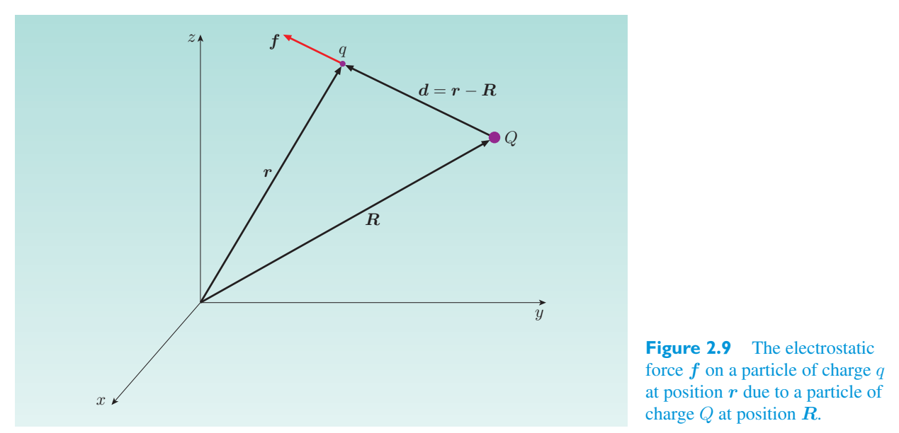
Knowledge of this force is useful only in some highly specific cases. What is generally of much greater value is knowledge of the electric field E (r). This is a vector field, meaning that it is a function of position that assigns a vector E to each point r throughout some region. At any point r, the assigned vector E is the force per unit charge that would act on a test charge q placed at r:对这种力的了解仅在某些非常具体的情况下才有用。通常更有价值的是电场 E (r) 的知识。这是一个向量场,意味着它是位置的函数,将向量 E 分配给整个某个区域的每个点 r。在任意点 r,指定的矢量 E 是作用于放置在 r 处的测试电荷 q 的每单位电荷的力:
So, once the electric field throughout some region has been determined, the electrostatic force on any test charge q introduced at a point r can be predicted using因此,一旦确定了整个某个区域的电场,就可以使用以下公式来预测在点 r 引入的任何测试电荷 q 上的静电力:
A similar approach may be taken to magnetic forces. This case is somewhat more complicated because the magnetic force on a charged particle generally depends on the particle’s velocity as well as its position and charge. For example, the force on a charge q moving with velocity v through a point r that is at a perpendicular distance d from a long straight wire carrying a current I is given by对于磁力可以采取类似的方法。这种情况稍微复杂一些,因为带电粒子上的磁力通常取决于粒子的速度及其位置和电荷。例如,以速度 v 穿过点 r 的电荷 q 上的力,该点与载有电流 I 的长直导线的垂直距离 d 为
where \(\mu\) 0 is the permeability of free space (an invariant constant with the value 4 \(\pi\) × 10 − 7 N m \(\mathrm{A^{-1}}\)) and \(\theta\) E is a unit vector at right angles to the wire, as indicated in Figure 2.10 overleaf. Note that the symbol × in Equation 2.80 indicates a vector product, so directions are very important if it is to be correctly interpreted.其中 \(\mu\) 0 是自由空间的磁导率(恒定常数,值为 4 \(\pi\) × 10 − 7 N m \(\mathrm{A^{-1}}\)),\(\theta\) E 是与导线成直角的单位向量,如背面图 2.10 所示。请注意,公式 2.80 中的符号 × 表示矢量积,因此如果要正确解释方向,方向非常重要。
Once again, it is useful to have a more general prescription for the force, and this again involves the introduction of a vector field — in this case the magnetic field B (r), which is defined so that at the point r,再一次,对力有一个更通用的规定是有用的,这又涉及到矢量场的引入——在本例中是磁场 B (r),其定义为在点 r,
Once the magnetic field has been determined throughout some region, the force on any test charge moving through that region can be predicted.一旦确定了某个区域的磁场,就可以预测移动穿过该区域的任何测试电荷所受的力。
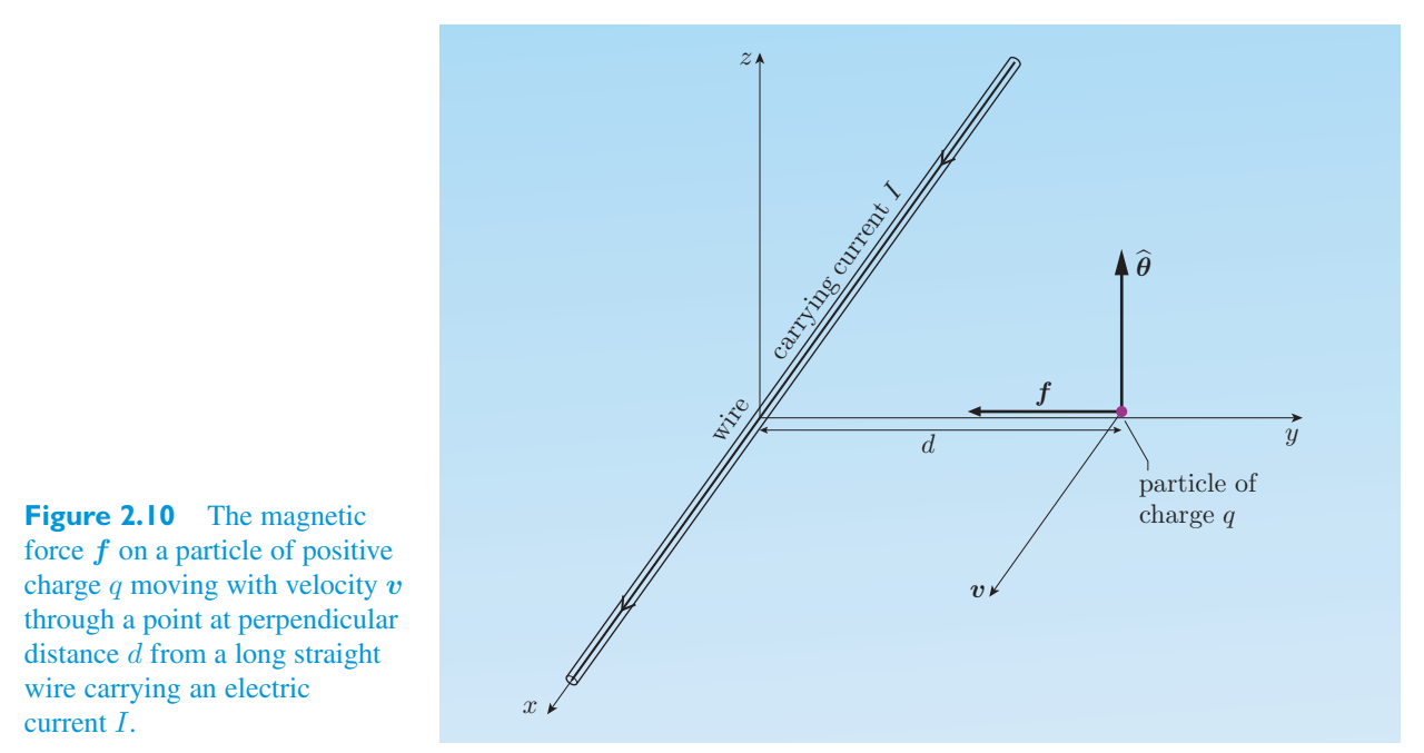
Combining these descriptions of electric and magnetic forces, we see that in a region where there is both an electric field and a magnetic field, the electromagnetic force on a particle of charge q travelling with velocity v is given by the Lorentz force law结合这些对电力和磁力的描述,我们看到,在同时存在电场和磁场的区域中,以速度 v 运动的电荷粒子 q 上的电磁力由洛伦兹力定律给出
The role of the vector product can be seen by writing out the individual components of the Lorentz force,通过写出洛伦兹力的各个分量可以看出矢量积的作用,
which can also be written in matrix form as也可以写成矩阵形式
Our aim now is to find a way of rewriting the Lorentz force law in a manifestly covariant way. We should expect the final result to include four-vectors such as the four-force and the four-velocity, but the complexity of the above expressions suggests that something more will be required. The key extra ingredient is a new multi-component entity called the electromagnetic four-tensor or sometimes simply the field tensor. This can be denoted [F \(\mu\)\(\nu\)] and will have 16 components F \(\mu\)\(\nu\) that may be identified from the following:我们现在的目标是找到一种以明显协变的方式重写洛伦兹力定律的方法。我们应该期望最终结果包括四向量,例如四力和四速度,但上述表达式的复杂性表明还需要更多的东西。关键的额外成分是一种新的多分量实体,称为电磁四张量,有时简称为场张量。这可以表示为 [F \(\mu\)\(\nu\)] 并且将具有 16 个分量 F \(\mu\)\(\nu\),可以通过以下方式识别:
It is unfortunate and potentially confusing that both the four-force and the field tensor are represented by an upper-case F, so we have used different typefaces for the two quantities. It may help that the field tensor will always have two indices while the four-force has only one. Nonetheless, you will need to take care not to confuse the two symbols.不幸的是,四力和场张量都由大写 F 表示,因此可能会造成混淆,因此我们对这两个量使用了不同的字体。场张量总是有两个索引,而四力只有一个索引,这可能会有所帮助。尽管如此,您需要注意不要混淆这两个符号。
Now, the truly remarkable thing about the electromagnetic four-tensor is that it behaves very simply under a Lorentz transformation. The positioning of the indices \(\mu\) and \(\nu\) in the raised contravariant location indicates the exact behaviour. If S and \(S'\) are two, inertial frames in standard configuration, with coordinates related by \(x'\) \(\mu\) = 3 \(\Lambda\) \(\mu\) x \(\nu\), then the field tensor components \(F'\) \(\mu\)\(\nu\) measured in frame \(S'\) will be related to those measured in frame S by现在,电磁四张量真正值得注意的是它在洛伦兹变换下的表现非常简单。索引 \(\mu\) 和 \(\nu\) 在凸起逆变位置的定位指示了确切的行为。如果 S 和 \(S'\) 是标准配置中的两个惯性坐标系,坐标由 \(x'\) \(\mu\) = 3 \(\Lambda\) \(\mu\) x \(\nu\) 相关,则在 \(S'\) 坐标系中测量的场张量分量 \(F'\) \(\mu\)\(\nu\) 将与在 S 坐标系中测量的场张量分量相关:
Given that the fully contravariant field tensor [F \(\mu\)\(\nu\)] does behave in this way, we can use the Minkowski metric to lower one of the indices, giving what is often referred to as the mixed version of the field tensor:鉴于完全逆变场张量 [F \(\mu\)\(\nu\)] 确实以这种方式表现,我们可以使用闵可夫斯基度规来降低其中一个索引,给出通常称为场张量的混合版本:
And then we can use the metric again to lower the remaining index, giving the fully covariant form:然后我们可以再次使用该度规来降低剩余索引,给出完全协变形式:
Performing the sums is tedious and needs care, but the process is straightforward and leads to the result进行求和是乏味且需要小心的,但过程很简单并且会得出结果
Once again we see that, superficially at least, all that the index lowering has achieved is the reversal of some signs; but the real significance is that the fully covariant form of the field tensor transforms differently from the fully contravariant form. Under a Lorentz transformation implemented by the transformation matrix [\(\Lambda\) \(\mu\) \(\nu\)], the fully covariant form transforms with the inverse Lorentz transformation matrix [(\(\Lambda\) − 1) \(\mu\) \(\nu\)] just as a derivative did. Specifically,我们再次看到,至少从表面上看,指数下调所带来的只是一些迹象的逆转;但真正的意义在于,场张量的完全协变形式与完全逆变形式的变换不同。在由变换矩阵 [\(\Lambda\) \(\mu\) \(\nu\)] 实现的洛伦兹变换下,完全协变形式与逆洛伦兹变换矩阵 [(\(\Lambda\) − 1) \(\mu\) \(\nu\)] 进行变换,就像导数一样。具体来说,
These transformations are of great interest in their own right, and their implications for the electric and magnetic fields will be discussed in the next subsection. For the moment, however, we shall simply note that the transformations involve products of elements of the Lorentz transformation matrix or its inverse, and concentrate on the implications of this for the Lorentz force law.这些变换本身就很有趣,它们对电场和磁场的影响将在下一小节中讨论。然而,目前我们只需注意变换涉及洛伦兹变换矩阵或其逆矩阵的元素的乘积,并集中讨论这对洛伦兹力定律的影响。
Now consider the following equation:现在考虑以下等式:
On the left is a contravariant four-force; on the right is the product of an invariant (q), a four-tensor with two contravariant indices (F \(\mu\)\(\nu\)) and a covariant four-vector (U \(\nu\)) — there is a contraction over one raised index and the lowered one. So the right-hand side has only one free index, and that is raised, just like the one free index on the left-hand side. The upshot of all this is that the equation is expressed entirely in terms of entities that transform in simple ways under a Lorentz transformation, and those entities are combined in such a way that both sides of the equation will transform in the same manner. In other words, the given equation is manifestly covariant under Lorentz transformation. (Incidentally, note that in the last sentence we are using ‘covariant’ in the sense of ‘form-invariant’, not in the sense of ‘transforming like a derivative’. It is unfortunate that the word is used in these two ways, but it is a customary practice.)左边是逆变四力;右边是一个不变量 (q)、一个具有两个逆变索引 (F \(\mu\)\(\nu\)) 的四张量和一个协变四向量 (U \(\nu\)) 的乘积 - 一个升高的索引和降低的索引存在收缩。因此,右侧只有一个空闲索引,并且该索引被提升,就像左侧的一个空闲索引一样。所有这一切的结果是,方程完全用在洛伦兹变换下以简单方式变换的实体来表达,并且这些实体以这样的方式组合,使得方程两边将以相同的方式变换。换句话说,给定的方程在洛伦兹变换下是明显协变的。(顺便说一句,请注意,在最后一句中,我们在“形式不变”的意义上使用“协变”,而不是“像导数一样变换”。不幸的是,这个词以这两种方式使用,但这是一种习惯做法。)
Of course, the real reason for our interest in Equation 2.90 is that it provides a covariant formulation of the Lorentz force law. You should convince yourself of this by actually performing the sum and checking the result, but the outcome can be more easily seen by interpreting the sum as the following matrix relationship (take the first index on any element to indicate the row):当然,我们对方程 2.90 感兴趣的真正原因是它提供了洛伦兹力定律的协变公式。您应该通过实际执行求和并检查结果来说服自己这一点,但是通过将求和解释为以下矩阵关系(采用任何元素上的第一个索引来指示行)可以更容易地看到结果:
Note that the v in this expression is the speed of the particle, the magnitude of the velocity v = (\(v_{x}\), \(v_{y}\), \(v_{z}\)). Also note that the negative signs in the right-hand column vector are there because it represents the covariant four-velocity. It is \(\gamma(v)\) on both sides, the clear from the matrix expression that, after cancelling a last three rows reproduce the component expressions of the Lorentz force law that were given earlier.注意,这个表达式中的 v 是粒子的速度,速度的大小 v = (\(v_{x}\), \(v_{y}\), \(v_{z}\))。另请注意,右侧列向量中的负号在那里,因为它代表协变四速度。两边都是 \(\gamma(v)\),从矩阵表达式可以清楚地看出,取消最后三行后,再现了前面给出的洛伦兹力定律的分量表达式。
What about the first row in the matrix equation? That is the equation矩阵方程的第一行呢?这就是等式
It tells us the rate at which the Lorentz force does work and thereby increases the total energy. It does not contain any surprises, but it reflects the well-known fact that only the electric field is effective in doing work on the particle; this is because the magnetic part of the Lorentz force always acts at right angles to the particle’s velocity.它告诉我们洛伦兹力做功的速率,从而增加总能量。它并不包含任何令人惊讶的内容,但它反映了一个众所周知的事实:只有电场才能有效地对粒子做功;这是因为洛伦兹力的磁性部分始终与粒子的速度成直角。
So we now have a second law of Lorentz-covariant electromagnetism.所以我们现在有了洛伦兹协变电磁学第二定律。
The covariant Lorentz force law协变洛伦兹力定律
Exercise 2.12 The, Lorentz force law may also be, expressed covariantly using练习 2.12 洛伦兹力定律也可以用协变的方式表示
the equation F = q 3 F U \(\nu\), but not F = q 3 F U \(\nu\). Why does the former work, but not the latter?方程 F = q 3 F U \(\nu\),但不是 F = q 3 F U \(\nu\)。为什么前者有效,而后者无效?
2.3.3 The transformation of electric and magnetic fields2.3.3 电场和磁场的变换
The ‘simple’ transformation law of the electromagnetic four-tensor is vital for the successful formulation of the Lorentz-covariant force law, but it is also of great interest in itself. In particular, it shows that electric and magnetic fields become mixed together in relativity, in a way that is not unlike the mixing of energy and momentum seen earlier. What is an electric field to an observer in frame S will be observed as a combination of electric and magnetic fields by an observer in frame \(S'\). In a relativistic universe, electric and magnetic phenomena are not completely separate. The existence of electric charge, combined with the requirements of special relativity, demands the existence of magnetism.电磁四张量的“简单”变换定律对于洛伦兹协变力定律的成功制定至关重要,但它本身也很有趣。特别是,它表明电场和磁场在相对论中混合在一起,其方式与之前看到的能量和动量的混合没有什么不同。对于 S 系中的观察者来说电场是什么,将被 S 系中的观察者观察到电场和磁场的组合。在相对论宇宙中,电现象和磁现象并不是完全分开的。电荷的存在,结合狭义相对论的要求,需要磁性的存在。
The transformation properties of electric and magnetic fields follow from the transformation properties of the field tensor. We already know that电场和磁场的变换性质源自场张量的变换性质。我们已经知道
and we know that in this fully contravariant case,我们知道,在这个完全逆变的情况下,
In the case where the Lorentz transformation matrix is the usual one, relating frames S and \(S'\) in standard configuration, the transformation is easier than it looks because many of the elements are zero. Even so, we shall not go through the details (you may do that if you wish), but we shall quote the result of a slightly more general Lorentz transformation in which frame \(S'\) has an arbitrary velocity V (not necessarily in the x -direction) in frame S. In this case the transformation rules are usually expressed for field components that are parallel在洛伦兹变换矩阵是通常的情况下,在标准配置中关联框架 S 和 \(S'\),变换比看起来更容易,因为许多元素为零。即便如此,我们不会详细介绍(如果您愿意,您可以这样做),但我们将引用稍微更一般的洛伦兹变换的结果,其中框架 \(S'\) 在框架 S 中具有任意速度 V(不一定在 x 方向)。在这种情况下,变换规则通常表示为平行的场分量
(indicated by 1) or perpendicular (indicated by ⊥) to the direction of V:(用 1 表示)或垂直于(用 ⊥ 表示)V 方向:
These equations beautifully illustrate the blending of electricity and magnetism that relativity demands. Looking back at the covariant Lorentz force law, you can see the electromagnetic four-tensor as the mathematical entity required to allow a velocity-dependent force to be consistent with Lorentz covariance. From this point of view, electromagnetism is as simple as it could be.这些方程完美地说明了相对论所要求的电和磁的混合。回顾协变洛伦兹力定律,您可以将电磁四张量视为允许与速度相关的力与洛伦兹协方差一致所需的数学实体。从这个角度来看,电磁学是非常简单的。
Exercise 2.13 Using Equation 2.85 and taking [\(\Lambda\) \(\mu\)练习2.13 使用公式2.85并取[\(\Lambda\) \(\mu\)
\(\nu\)] to represent the usual Lorentz transformation between frames in standard configuration, show that \(E'\) = E.\(\nu\)] 代表标准配置中框架之间通常的洛伦兹变换,表明 \(E'\) = E。
2.3.4 The Maxwell equations2.3.4 麦克斯韦方程组
The remaining laws of vacuum electromagnetism are the Maxwell equations. These are the laws that determine the electric and magnetic fields in a given region. They relate the electric and magnetic fields to the charge and current densities that are their sources, and also to each other since a changing magnetic field can produce an electric field, and a changing electric field can produce a magnetic field.真空电磁学的其余定律是麦克斯韦方程组。这些定律决定了给定区域的电场和磁场。它们将电场和磁场与其来源的电荷和电流密度相关联,并且也将它们彼此相关联,因为变化的磁场可以产生电场,而变化的电场可以产生磁场。
In elementary treatments, the Maxwell equations are usually presented as a set of four differential equations written in the compact language of vector calculus, or sometimes as the equivalent set of eight component equations. This book does not assume any detailed familiarity with the Maxwell equations. The vector calculus versions are shown below, but all that matters mathematically is that the left-hand sides of the equations represent various combinations of partial derivatives of the electric and magnetic field components with respect to the spatial coordinates x, y and z:在初等处理中,麦克斯韦方程通常表示为一组用向量微积分的紧凑语言编写的四个微分方程组,或者有时表示为一组八个分量方程组。本书不假设您对麦克斯韦方程有任何详细的了解。矢量微积分版本如下所示,但在数学上最重要的是方程的左侧表示电场和磁场分量相对于空间坐标 x、y 和 z 的偏导数的各种组合:
where ∇ represents the vector derivative其中 ∇ 表示向量导数
The invariant constants that appear in these equations are not independent. They are linked by the equation \(\mu\) 0 ε 0 \(c^2\) = 1.这些方程中出现的不变常数不是独立的。它们通过方程 \(\mu\) 0 ε 0 \(c^2\) = 1 联络。
The charge and current densities were introduced earlier as components of the current four-vector. The fields, of course, are components of the electromagnetic four-tensor. The way to covariantly construct eight component equations from these ingredients is as follows.电荷和电流密度之前作为电流四矢量量量的组成部分引入。当然,场是电磁四张量的组成部分。从这些成分协变构造八分量方程的方法如下。
The covariant Maxwell equations协变麦克斯韦方程组
The first of these covariant equations has one free index and represents four component equations. These include references to the charge density and the current density, and reproduce Equations 2.97 and 2.100. The interpretation of the second covariant equation is less clear. It has three free indices, which indicates 64 (= 4 × 4 × 4) component equations. However, if any two of the indices are the same, the equation concerned is identically zero. Furthermore, in those cases where all the indices are different, permutations such as \(\lambda\) = 1, \(\mu\) = 2, \(\nu\) = 3 and \(\lambda\) = 2, \(\mu\) = 3, \(\nu\) = 1 lead to the same equation. Taking these symmetries into account, the original 64 component equations are reduced to just four independently meaningful equations. This second set of four component equations reproduces Equations 2.98 and 2.99. Thus, taken together, the two covariant equations reproduce the complete set of Maxwell equations and conclude our rewriting of the laws of vacuum electromagnetism in a manifestly covariant form. All that remains is to draw some lessons that will be of value in future chapters.这些协变方程中的第一个有一个自由索引并表示四个分量方程。其中包括对电荷密度和电流密度的引用,并重现方程 2.97 和 2.100。第二个协变方程的解释不太清楚。它有 3 个自由索引,表示 64 (= 4 × 4 × 4) 个分量方程。然而,如果任意两个指数相同,则相关方程同样为零。此外,在所有索引都不同的情况下,诸如 \(\lambda\) = 1、\(\mu\) = 2、\(\nu\) = 3 和 \(\lambda\) = 2、\(\mu\) = 3、\(\nu\) = 1 等排列会导致相同的方程。考虑到这些对称性,原来的 64 个分量方程被简化为只有 4 个独立有意义的方程。第二组四分量方程再现了方程 2.98 和 2.99。因此,两个协变方程合在一起再现了完整的麦克斯韦方程组,并以明显的协变形式得出了我们对真空电磁定律的重写结论。剩下的就是吸取一些在以后的章节中有价值的教训。
2.3.5 Four-tensors2.3.5 四张量
Exposing the formal simplicity, almost the inevitability, of electromagnetism is one of the great triumphs of special relativity. However, from the point of view of relativity itself, the main development in this chapter has been the introduction of tensors. In this particular chapter the tensors have been called four-tensors. This indicates that they are specific to special relativity. You will meet a much more general class of tensors later, when we move on to general relativity, but a good understanding of four-tensors will be a valuable starting point for that more general experience.揭示电磁学的形式简单性,几乎是必然性,是狭义相对论的伟大胜利之一。然而,从相对论本身的角度来看,本章的主要发展是张量的引入。在这一章中,张量被称为四张量。这表明它们特定于狭义相对论。稍后,当我们转向广义相对论时,您将遇到更一般的张量类别,但是对四张量的良好理解将是更一般经验的宝贵起点。
The only four-tensor that we have formally introduced so far is the electromagnetic four-tensor [F \(\mu\)\(\nu\)] and its variants \([F^{\mu}]\) and [F], but you have already met some others. For instance, the vitally important Minkowski metric [\(\eta\) \(\mu\)\(\nu\)] is a fully covariant four-tensor, and the quantity [\(\eta\) \(\mu\)\(\nu\)] is a fully contravariant four-tensor. Moreover, the term four-tensor is used in such a general sense that these two-indexed examples represent only one particular class of four-tensors — technically referred to as four-tensors of rank 2. All four-vectors are also four-tensors, but they are of rank 1, and it is easy to define four-tensors of rank 3, rank 4, or any higher rank.到目前为止,我们正式介绍的唯一四张量是电磁四张量 [F \(\mu\)\(\nu\)] 及其变体 \([F^{\mu}]\) 和 [F],但您已经遇到了其他一些。例如,极其重要的闵可夫斯基度规 [\(\eta\) \(\mu\)\(\nu\)] 是一个完全协变的四张量,而数量 [\(\eta\) \(\mu\)\(\nu\)] 是一个完全逆变的四张量。此外,术语“四张量”在一般意义上使用,即这些两个索引的示例仅代表一类特定的四张量 - 技术上称为 2 阶四张量。所有四向量也是四张量,但它们的阶为 1,并且很容易定义 3 阶、4 阶或任何更高阶的四张量。
The defining characteristic of any four-tensor, whatever its rank, is its behaviour under Lorentz transformations. If S and \(S'\) are two inertial frames linked by a general Lorentz transformation (i.e. not necessarily in standard configuration), then we, know that the coordinates in S will be related to those in \(S'\) by [\(\Lambda\) \(\mu\)]\([x^{\nu}]\). (Note that we are now using \(\Lambda\) \(\mu\) in a more general sense than before; we shall have to clarify this shortly.) Under such a general Lorentz rank m consists of 4 m transformation, a four-tensor [T \(\mu\) 1,\((\mu)^2\),...,\(\mu\) m] of contravariant components that transform according to任何四张量的定义特征,无论其等级如何,都是其在洛伦兹变换下的行为。如果 S 和 \(S'\) 是通过一般洛伦兹变换(即不一定在标准配置中)联络的两个惯性系,那么我们知道 S 中的坐标将通过 [\(\Lambda\) \(\mu\)]\([x^{\nu}]\) 与 \(S'\) 中的坐标相关。(请注意,我们现在使用的 \(\Lambda\) \(\mu\) 比以前更广泛;我们必须尽快澄清这一点。)在这样的一般洛伦兹秩 m 包含 4 m 变换下,逆变分量的四张量 [T \(\mu\) 1,\((\mu)^2\),...,\(\mu\) m] 根据以下公式进行变换
Under the same Lorentz transformation, a covariant four-tensor of rank n is a collection of 4 n components that transform according to在相同的洛伦兹变换下,秩为 n 的协变四张量是 4 n 个分量的集合,这些分量根据以下公式进行变换
where [(\(\Lambda\) − 1) \(\mu\) \(\nu\)] is the matrix inverse of [\(\Lambda\) \(\mu\) \(\nu\)] in the usual sense that其中 [(\(\Lambda\) − 1) \(\mu\) \(\nu\)] 是通常意义上的 [\(\Lambda\) \(\mu\) \(\nu\)] 的矩阵逆
A mixed four-tensor of contravariant rank m and covariant rank n consists of 4 m + n components that transform according to逆变秩 m 和协变秩 n 的混合四张量由 4 m + n 个分量组成,这些分量根据以下公式进行变换
All that remains is to specify the elements of the general Lorentz transformation matrix that is the basis of this general definition of a four-tensor. We already \(\Lambda\) 0 0 = \(\gamma(V)\), know that if S and \(S'\) are in standard configuration, then \(\Lambda\) 0 = − \(\gamma(V)\) V/c, \(\Lambda\) 1 = − \(\gamma(V)\) V/c and \(\Lambda\) 1 = \(\gamma(V)\), but what if the inertial frames S and \(S'\) are not in standard configuration? What if the axes are not aligned, for example, or the origin of \(S'\) never passes through the origin of S? What form do the matrix elements take under such general circumstances? We saw earlier, when deriving the Lorentz transformations in Chapter 1, that the primed coordinates have to be linear functions of the unprimed coordinates. In such circumstances, the constants that determine the transformation, the generalized analogues of \(\gamma(V)\) and \(\gamma(V)\) V/c, can be represented by partial derivatives of the coordinates, so the elements of the general Lorentz transformation matrix can be written as剩下的就是指定一般洛伦兹变换矩阵的元素,该矩阵是四张量一般定义的基础。我们已经 \(\Lambda\) 0 0 = \(\gamma(V)\),知道如果 S 和 \(S'\) 处于标准配置,则 \(\Lambda\) 0 = − \(\gamma(V)\) V/c,\(\Lambda\) 1 = − \(\gamma(V)\) V/c 和 \(\Lambda\) 1 = \(\gamma(V)\),但是如果惯性呢?车架S和\(S'\)不是标准配置吗?例如,如果轴未对齐,或者 \(S'\) 的原点从未经过 S 的原点,该怎么办?在这种一般情况下矩阵元素采取什么形式?我们之前在第一章推导洛伦兹变换时看到,带底数的坐标必须是未带底数的坐标的线性函数。在这种情况下,决定变换的常数,即 \(\gamma(V)\) 和 \(\gamma(V)\) V/c 的广义类似物,可以用坐标的偏导数来表示,因此一般洛伦兹变换矩阵的元素可以写为
and the elements of the corresponding inverse transformation will be相应逆变换的元素为
Substituting these expressions into Equation 2.107 gives将这些表达式代入公式 2.107 得出
This is the form of the general tensor transformation law that you will meet later. The main difference is that in the case of four-tensors and special relativity, the partial derivatives are all constants that are independent of spacetime position. This will not always be the case in general relativity, as will soon become clear.这就是稍后您将遇到的一般张量变换定律的形式。主要区别在于,在四张量和狭义相对论的情况下,偏导数都是与时空位置无关的常数。在广义相对论中,情况并不总是如此,这一点很快就会变得清楚。
Exercise 2.14 You are told that the 256 -component object [H \(\mu\)\(\nu\)\(\rho\)\(\eta\)] with练习 2.14 你被告知 256 分量对象 [H \(\mu\)\(\nu\)\(\rho\)\(\eta\)] 与
elements H \(\mu\)\(\nu\)\(\rho\)\(\eta\) is a fully covariant four-tensor of rank 4. Write down the general rule for transforming its components from frame S to frame \(S'\).elements H \(\mu\)\(\nu\)\(\rho\)\(\eta\) 是一个完全协变的 4 阶四张量。写下将其分量从框架 S 转换到框架 \(S'\) 的一般规则。
Summary of Chapter 2第 2 章总结
1. Invariants that take the same value in all inertial frames include the speed of1. 在所有惯性系中取相同值的不变量包括
light in a vacuum, the spacetime separation between events, the proper time between time-like separated events, the charge of a particle and the mass of a particle.真空中的光、事件之间的时空分离、类似时间的分离事件之间的固有时间、粒子的电荷和粒子的质量。
2. The principle of relativity demands that the laws of physics should be2. 相对性原理要求物理定律应该是
form-invariant under Lorentz transformations. Such laws are said to be Lorentz-covariant.洛伦兹变换下的形式不变。这些定律被称为洛伦兹协变。
3. The relativistic momentum of a particle of mass m and velocity v is3. 质量为 m、速度为 v 的粒子的相对论动量为
4. The relativistic kinetic energy of a particle of mass m and speed v is4. 质量为 m、速度为 v 的粒子的相对论动能为
5. The total relativistic energy of a particle of mass m and speed v is5. 质量为 m、速度为 v 的粒子的总相对论能量为
where \(E_0\) = \(mc^2\) is the mass energy of the particle.其中 \(E_0\) = mc 2 是粒子的质量能。
6. In the absence of external forces, relativistic total energy is conserved, but6.在没有外力的情况下,相对论总能量守恒,但
neither kinetic energy nor mass energy is necessarily conserved. This establishes an ‘equivalence’ of mass and energy, with many important consequences.neither kinetic energy nor mass energy is necessarily conserved.这建立了质量和能量的“等价”,并产生许多重要的后果。
7. The four-momentum \([P^{\mu}]\) = (E/c, p, p, p) brings together momentum7. 四动量 \([P^{\mu}]\) = (E/c, p, p, p) 汇聚动量
and energy. It transforms in the same way as a four-displacement:和能量。它的变形方式与四排量相同:
m is米是
8. The energy–momentum relation for a particle of mass8. 质量粒子的能量-动量关系
showing that for a massless particle p = E/c.表明对于无质量粒子 p = E/c。
9. Laws of conservation of total energy and momentum9.总能量和动量守恒定律
are combined in a manifestly covariant law of four-momentum conservation.结合在一个明显的四动量守恒协变定律中。
10. The four-force \([F^{\mu}]\) = ((γ/c) f · v, γ f) determines10. 四力 \([F^{\mu}]\) = ((γ/c) f · v, γ f) 确定
the rate of change of a particle’s four-momentum with respect to proper time. It transforms like the four-momentum, placing restrictions on the acceptable expressions for the three-force f. The electromagnetic Lorentz force meets these requirements; Newton’s gravitational force does not. 3 \(\nu\) =0 \(\Lambda\) \(\mu\) \(\nu\) x \(\nu\), a粒子四动量相对于原时间的变化率。它像四动量一样变换,对三力 f 的可接受表达式施加限制。电磁洛伦兹力满足这些要求;牛顿的万有引力则不然。 3 \(\nu\) =0 \(\Lambda\) \(\mu\) \(\nu\) x \(\nu\),一个
11. Under a Lorentz transformation in which \(x'\) \(\mu\) =11. 在洛伦兹变换下,其中 \(x'\) \(\mu\) =
contravariant four-vector \([A^{\mu}]\) transforms in the same way as a four-displacement:逆变四向量 \([A^{\mu}]\) 的变换方式与四位移相同:
Under the same Lorentz transformation, a covariant transforms in the same way as a set of derivatives:在相同的洛伦兹变换下,协变的变换方式与一组导数相同:
where [(\(\Lambda\) − 1) \(\mu\) \(\nu\)] is the matrix inverse of [\(\Lambda\) \(\mu\) \(\nu\)]. In the case of two frames in standard configuration,其中 [(\(\Lambda\) − 1) \(\mu\) \(\nu\)] 是 [\(\Lambda\) \(\mu\) \(\nu\)] 的矩阵逆。标准配置两框的情况下,
12. Indices on four-vectors may be lowered or raised12. 四向量指数可降低或提高
using the, Minkowski by \(\nu\) \(\eta\) \(\alpha\)\(\nu\) \(\eta\) \(\nu\)\(\beta\) = δ \(\alpha\) \(\beta\): metric \(\eta\) \(\mu\)\(\nu\) or the related inverse quantity \(\eta\) \(\mu\)\(\nu\) defined使用闵可夫斯基通过 \(\nu\) \(\eta\) \(\alpha\)\(\nu\) \(\eta\) \(\nu\)\(\beta\) = δ \(\alpha\) \(\beta\):公制 \(\eta\) \(\mu\)\(\nu\) 或相关的反数量\(\eta\) \(\mu\)\(\nu\) 已定义
and和
13. Contraction involves summing over one raised and13. 收缩涉及将一个升高的和
one lowered index, and may be used to form invariants as in一个降低的索引,可用于形成不变量,如
14. The Lorentz-covariant laws of electromagnetism are:14. 电磁学的洛伦兹协变定律是:
the covariant equation of continuity连续性协变方程
the covariant Lorentz force law协变洛伦兹力定律
the covariant Maxwell equations协变麦克斯韦方程组
where \([J^{\mu}]\) = (cρ, J, J, J) is the contravariant current four-vector, and [F \(\mu\)\(\nu\)] is the fully contravariant electromagnetic four-tensor given by其中 \([J^{\mu}]\) = (cρ, J, J, J) 是逆变电流四矢量量量,[F \(\mu\)\(\nu\)] 是完全逆变电磁四张量,由下式给出
15. Under a Lorentz transformation, the electromagnetic four-tensor transforms15. 在洛伦兹变换下,电磁四张量变换
according to根据
This leads to the following transformation laws for the electric and magnetic fields:这导致了以下电场和磁场的变换定律:
16. Under a general Lorentz transformation, the components of a four-tensor16. 在一般洛伦兹变换下,四张量的分量
transform according to变换根据
Chapter 3 Geometry and curved spacetime第三章几何与弯曲时空
Introduction介绍
Einstein’s 1905 theory of special relativity concerns relationships between observations made by inertial observers in uniform relative motion. As you saw in the previous chapter, the theory is inconsistent with Newtonian gravitation. In 1907, in what he later described as ‘the happiest thought of my life’, Einstein realized that a theory of general relative motion — one that included relationships between observations made by accelerated observers — would also shed light on the problem of gravitation. It was not long after this that Minkowski introduced his four-dimensional spacetime approach to special relativity, which revealed the geometric basis of the theory. Under these influences, Einstein’s own thinking took on an increasingly geometric flavour, and by the middle of 1912 he realized that to make further progress in relativity and gravitation, he needed to find out what mathematicians knew about certain problems concerning invariants in geometry. At that point he asked his friend, the mathematician Marcel Grossman (1878–1936), to help him to find the required information. Grossman was soon able to tell Einstein that what he was looking for was contained in the subject known as Riemannian geometry — a branch of mathematics particularly concerned with the study of curved spaces.爱因斯坦 1905 年提出的狭义相对论关注的是惯性观察者在匀速相对运动中所做的观察之间的关系。正如您在上一章中看到的,该理论与牛顿引力不一致。1907 年,爱因斯坦意识到广义相对运动理论(包括加速观察者的观测结果之间的关系)也将揭示引力问题,后来他将其描述为“我一生中最幸福的想法”。不久之后,闵可夫斯基将他的四维时空方法引入了狭义相对论,揭示了该理论的几何基础。在这些影响下,爱因斯坦自己的思想越来越带有几何色彩,到1912年中期,他意识到,为了在相对论和万有引力方面取得进一步进展,他需要了解数学家对几何不变量的某些问题的了解。此时,他请他的朋友、数学家马塞尔·格罗斯曼(Marcel Grossman,1878-1936)帮助他找到所需的信息。格罗斯曼很快就告诉爱因斯坦,他正在寻找的东西包含在被称为黎曼几何的学科中——这是一个特别关注弯曲空间研究的数学分支。
Geometry is the study of shape and spatial relationships. The kind of geometry taught in high schools is known as Euclidean geometry, after Euclid of Alexandria who collected together the main results of the field in around 300 BC. Among the best known of those results (see Figure 3.1) are:几何学是对形状和空间关系的研究。高中教授的几何学被称为欧几里得几何,得名于亚历山大的欧几里得,他在公元前 300 年左右收集了该领域的主要成果。其中最著名的结果(见图 3.1)包括:
- • the internal angles of a triangle add up to 180 ◦• 三角形的内角之和为 180 °
- • a circle of radius R has a circumference of length C• 半径为 R 的圆的周长为 C
- • a sphere of radius R has a surface area A = 4 πR 2.• 半径为 R 的球体的表面积 A = 4 πR 2。
It was long thought that Euclidean geometry was the only kind of geometry, and that these results would therefore apply to all triangles, circles and spheres. mathematicians, Ja´nos However, in the first half of the nineteenth century, three Bolyai (1802–1860), Nikolai Lobachevsky (1792–1856), and Carl Friedrich Gauss (1777–1855; Figure 3.2), independently established that it was possible to formulate a kind of geometry that made mathematical sense but was quite different from traditional Euclidean geometry. In non-Euclidean geometry, none of the Euclidean results quoted above is necessarily true.长期以来,人们一直认为欧几里得几何是唯一的几何类型,因此这些结果适用于所有三角形、圆形和球体。然而,在十九世纪上半叶,三位博利亚伊(Bolyai,1802-1860)、尼古拉·洛巴切夫斯基(Nikolai Lobachevsky,1792-1856)和卡尔·弗里德里希·高斯(Carl Friedrich Gauss,1777-1855;图 3.2)独立地确立了建立一种具有数学意义但又与传统欧几里得几何截然不同的几何的可能性。在非欧几里德几何中,上面引用的欧几里德结果都不一定是正确的。
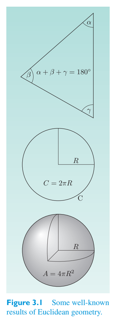
The realization that there was more than one kind of geometry meant that determining the geometric properties of the space around us was an experimental question, not just a mathematical one. Lobachevsky considered the possibility of using astronomical measurements to determine the true geometry of space, but concluded that they would not be sufficiently accurate. Gauss became involved in a land survey and examined the angles of the large triangle between three mountain tops. He failed to find any sign of non-Euclidean geometry, but he too realized that this might simply reflect the limited sensitivity of the technique that he was using.认识到存在不止一种几何形状意味着确定我们周围空间的几何特性是一个实验问题,而不仅仅是一个数学问题。罗巴切夫斯基考虑了使用天文测量来确定空间真实几何形状的可能性,但得出的结论是它们不够准确。高斯参与了一次土地测量,并检查了三个山顶之间的大三角形的角度。他未能找到任何非欧几里得几何的迹象,但他也意识到这可能只是反映了他所使用的技术的有限灵敏度。
Gauss was one of the greatest of all mathematicians. His many discoveries included several important contributions to the development of geometry. Not least was his part in helping to found differential geometry, the branch of mathematics that applies the techniques of calculus to the analysis of geometric problems. It was in furthering this subject that Gauss’s assistant Bernhard Riemann (1826–1866; Figure 3.3) introduced the geometry that now bears his name.高斯是最伟大的数学家之一。他的许多发现包括对几何学发展的几项重要贡献。尤其重要的是,他帮助建立了微分几何,这是将微积分技术应用于几何问题分析的数学分支。正是在进一步推进这一主题的过程中,高斯的助手伯恩哈德·黎曼(Bernhard 黎曼,1826-1866;图 3.3)引入了现在以他的名字命名的几何学。
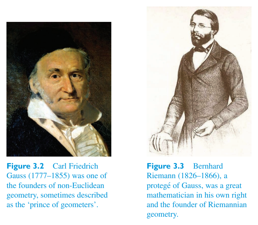
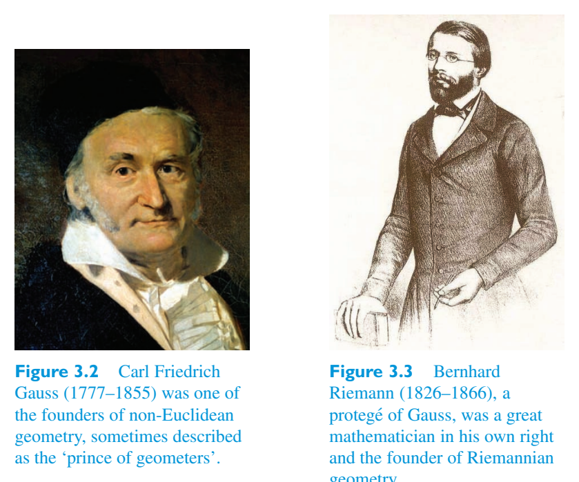
Riemann (1826–1866), a protege´ of Gauss, was a great mathematician in his own right and the founder of Riemannian geometry.黎曼(1826-1866)是高斯的弟子,也是一位伟大的数学家,也是黎曼几何的创始人。
has been properly explained, it will be sufficient to think of a ‘flat’ space as one in which the conventional Euclidean geometrical results hold true, and a ‘curved’ space as one in which they fail. Note that the terms ‘flat’ and ‘curved’ are used to describe geometric properties and may be applied to spaces with any number of dimensions. They do not simply mean ‘curved like a bow’ or ‘flat like a pancake’.已经得到了正确的解释,将“平坦”空间视为传统欧几里得几何结果成立的空间,将“弯曲”空间视为它们失败的空间就足够了。请注意,术语“平坦”和“弯曲”用于描述几何属性,并且可以应用于具有任意维数的空间。它们不仅仅意味着“像弓一样弯曲”或“像煎饼一样平坦”。
3.1 Line elements and differential geometry3.1 线元和微分几何
3.1.1 Line elements in a plane3.1.1 平面内的线单元
In order to analyze the geometry of curved space, we need to clarify what we mean by the length of a curve. Figure 3.4 shows a smooth curve C linking two points P and Q in an ordinary (Euclidean) plane. The plane is equipped with Cartesian coordinates so that each point on the curve can be assigned coordinates (x, y). The length of the curve can be approximately determined by dividing it into n short segments, each of which can be regarded as a straight line of length \(\Delta l\) (i = 1, 2,..., n), and then adding together the lengths of all those short straight lines. The approximate length of the curve C from P to Q will then be given by为了分析弯曲空间的几何形状,我们需要澄清曲线长度的含义。图 3.4 显示了在普通(欧几里得)平面中联络两点 P 和 Q 的平滑曲线 C。该平面配备有笛卡尔坐标,因此曲线上的每个点都可以指定坐标(x,y)。曲线的长度可以通过将其分成 n 个短段来近似确定,每个短段可以视为长度为 \(\Delta l\) (i = 1, 2,..., n) 的直线,然后将所有这些短直线的长度相加。从 P 到 Q 的曲线 C 的近似长度将由下式给出
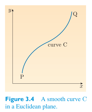
According to Pythagoras’s theorem, which is one of the fundamental results of Euclidean geometry, the length \(\Delta l\) of the straight line linking two points separated by the coordinate intervals \(\Delta x\) and \(\Delta y\) (see Figure 3.5) is given by根据毕达哥拉斯定理(欧几里德几何的基本结果之一),联络由坐标间隔 \(\Delta x\) 和 \(\Delta y\) 分隔的两点的直线长度 \(\Delta l\)(见图 3.5)由下式给出:
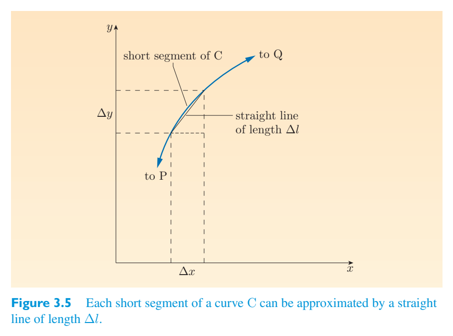
Decreasing the length of those short segments will increase their number and improve the accuracy of the approximation to the total length of C. Taking the limit as \(\Delta x\) → 0 and \(\Delta y\) → 0, the sum will become an integral, and we can write the length of curve C from P to Q as减少这些短线段的长度会增加它们的数量,提高逼近C总长度的精度。以Δ x→0和Δ y→0为极限,其和将成为一个积分,我们可以将曲线C从P到Q的长度写为
where the line element, d l, is defined by其中线元素 d l 定义为
or或者
Unfortunately, this is not enough to let us actually work out the length of C; we need to know how to perform such an integral. In particular, in order to add up all the line elements along the curve, we need to take account of their differing directions, which will cause each element d l to correspond to differently-sized increments in the x - and y -directions.不幸的是,这还不足以让我们实际计算出 C 的长度;我们需要知道如何进行这样的积分。特别是,为了将沿曲线的所有线元素相加,我们需要考虑它们的不同方向,这将导致每个元素 d l 对应于 x 和 y 方向上不同大小的增量。
One powerful way of taking the shape of C into account involves representing it as a parameterized curve. This requires that every point on the curve should be identified with a unique value of some continuously varying parameter, u say, so that the x - and y -coordinates of any particular point on the curve represent specific values of two coordinate functions x (u) and y (u) that effectively define the curve. So, for example:考虑 C 形状的一种有效方法是将其表示为参数化曲线。这要求曲线上的每个点都应该用某个连续变化的参数 u 的唯一值来标识,以便曲线上任何特定点的 x 和 y 坐标代表有效定义曲线的两个坐标函数 x (u) 和 y (u) 的特定值。因此,例如:
- • the parabola y = \(x_{2}\) can be described in terms of a parameter u by the抛物线 y = \(x_{2}\) 可以用参数 u 来描述:
functions x (u) = u, y (u) = \(u^{2}\)函数 x (u) = u, y (u) = \(u^{2}\)
- • the circle \(x_{2}\) + \(y^{2}\) = 1 can be described in terms of a parameter u by the圆 \(x_{2}\) + \(y^{2}\) = 1 可以用参数 u 来描述:
functions x (u) = cos(u), y (u) = sin(u).函数 x (u) = cos(u), y (u) = sin(u)。
(Notice how in the first example, it is easy to parameterize a single-valued function y = f (x): we just write x (u) = u and y (u) = f (u).)(请注意,在第一个示例中,参数化单值函数 y = f (x) 很容易:我们只需写 x (u) = u 和 y (u) = f (u)。)
Adopting this parametric approach, it’s clear that any two points on the curve C that are separated by coordinate intervals \(\Delta x\) and \(\Delta y\), will also be separated by some corresponding parameter interval \(\Delta u\), and we can say that采用这种参数化方法,很明显,曲线 C 上被坐标区间 \(\Delta x\) 和 \(\Delta y\) 分开的任何两点,也将被某个相应的参数区间 \(\Delta u\) 分开,我们可以说
and和
As \(\Delta u\) → 0 (so that \(\Delta x\) → 0 and \(\Delta y\) → 0), the fractions \(\Delta x\)/\(\Delta u\) and \(\Delta y\)/\(\Delta u\) become the derivatives d x/d u and d y/d u of x (u) and y (u) with respect to u, and it follows that当 \(\Delta u\) → 0(使得 \(\Delta x\) → 0 和 \(\Delta y\) → 0)时,分数 \(\Delta x\)/\(\Delta u\) 和 \(\Delta y\)/\(\Delta u\) 变为 x (u) 和 y (u) 对 u 的导数 d x/d u 和 d y/d u,得出
and hence, from Equation 3.5,), y (u)) to So, finally, the length of the curve C from P = (x (u Q = (x (u), y (u)) is given by the following.因此,从方程 3.5,), y (u)) 到 So,最后,由 P = (x (u Q = (x (u), y (u))) 得出的曲线 C 的长度由下式给出。
Length of a curve in a Euclidean plane欧几里得平面中曲线的长度
Once we know the functions x (u) and y (u) that parameterize the curve C, and the values of u that correspond to the points P and Q, this expression for the length of a curve between two points in a Euclidean plane really can be evaluated. It is our first major result in this chapter.一旦我们知道参数化曲线 C 的函数 x (u) 和 y (u),以及对应于点 P 和 Q 的 u 值,就可以真正评估欧几里得平面中两点之间的曲线长度表达式。这是我们本章的第一个主要成果。
Worked Example 3.1工作示例 3.1
(a) Parameterize the straight line y = 2(6 x + 1).(a) 参数化直线 y = 2(6 x + 1)。
(b) Using the line element method described above, calculate the length of the line from (0, 2) to (5, 14). Check your result using Pythagoras’s theorem.(b) 使用上述线元法,计算从 (0, 2) 到 (5, 14) 的线段长度。使用毕达哥拉斯定理检查您的结果。
Solution解决方案
is x = u, (a) This is a single-valued function, so a suitable parameterization y = 2(6 u + 1).是 x = u, (a) 这是一个单值函数,因此合适的参数化 y = 2(6 u + 1)。
(b) Differentiating with respect to u, we obtain(b) 对 u 求导,我们得到
Since x = u, we have u (0, 2) = 0 and u (5, 14) = 5, so Equation 3.6 gives由于 x = u,我们有 u (0, 2) = 0 和 u (5, 14) = 5,因此方程 3.6 给出
Pythagoras’s theorem gives the same answer:毕达哥拉斯定理给出了同样的答案:
Worked Example 3.2工作示例 3.2
Parameterize the circle \(x_{2}\) + \(y^{2}\) = \(R^2\), and find the length of the circumference in terms of the (constant) radius R.将圆 \(x_{2}\) + \(y^{2}\) = \(R^2\) 参数化,并根据(常数)半径 R 求出圆周的长度。
Solution解决方案
x (u) = R cos(u) and The simplest way to parameterize the circle is to set y (u) = R sin(u), as given earlier. Differentiating with respect to u, we obtainx (u) = R cos(u) 并且参数化圆的最简单方法是设置 y (u) = R sin(u),如前所述。对 u 求导,我们得到
To get the circumference C, we need to let u vary from 0 to 2 \(\pi\), so using \(\sin^2 u\) + \(\cos^2 u\) = 1, we have为了得到周长 C,我们需要让 u 在 0 到 2 \(\pi\) 之间变化,因此使用 \(\sin^2 u\) + \(\cos^2 u\) = 1,我们有
Exercise 3.1 (a) Sketch the curve parameterized by x = 3 \(u^{2}\), y = 4 \(u^{2}\). (b) Calculate the length L of the curve from u = 0 to u = 3.练习 3.1 (a) 绘制由 x = 3 \(u^{2}\), y = 4 \(u^{2}\) 参数化的曲线。 (b) 计算从 u = 0 到 u = 3 的曲线长度 L。
There are always many ways to parameterize a curve, but it is usually best to choose the simplest. For example, in Exercise 3.1 we used the parameterization x = 3 \(u^{2}\), y = 4 \(u^{2}\), but this gives us no particular benefit and it would be simpler to use x = 3 u, y = 4 u. For the circle in Worked Example 3.2, another possibility is x = u, y = ± (\(R^2\) − \(u^{2}\)) 1/2, but this would make the calculations much more difficult.参数化曲线的方法总是有很多种,但通常最好选择最简单的。例如,在练习 3.1 中,我们使用了参数化 x = 3 \(u^{2}\), y = 4 \(u^{2}\),但这并没有给我们带来特别的好处,而且使用 x = 3 u, y = 4 u 会更简单。对于工作示例 3.2 中的圆,另一种可能性是 x = u, y = ± (\(R^2\) – \(u^{2}\)) 1/2,但这会使计算变得更加困难。
When dealing with a general curve in the plane, instead of Cartesian coordinates, it is often more convenient to use plane polar coordinates (r, \(\phi\)), which can be defined in terms of (x, y) by当处理平面上的一般曲线时,使用平面极坐标 (r, \(\phi\)) 代替笛卡尔坐标通常更方便,它可以用 (x, y) 来定义:
as shown in Figure 3.6. Note that r is now a variable (not the constant radius R of Worked Example 3.2), so we can define any point in the plane by the coordinates (r, \(\phi\)), where r is the distance from the origin measured along a line that makes an angle \(\phi\) with the x -axis.如图3.6所示。请注意,r 现在是一个变量(不是工作示例 3.2 中的恒定半径 R),因此我们可以通过坐标 (r, \(\phi\)) 定义平面中的任何点,其中 r 是沿着与 x 轴形成角度 \(\phi\) 的直线测量到的距原点的距离。
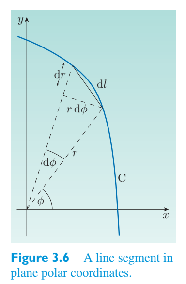
Using the rule for differentiating a product, it follows from the above definitions that使用区分产品的规则,从上述定义可以得出:
and so, from Equation 3.4, the line element in a Euclidean plane is also given by因此,根据方程 3.4,欧几里得平面中的线元素也由下式给出
This too is indicated in Figure 3.6.图 3.6 也表明了这一点。
Exercise 3.2 Use the parameterization r = R(a constant) and \(\phi\) = u练习 3.2 使用参数化 r = R(常数)和 \(\phi\) = u
(a variable parameter) together with Equation 3.7 to again find the circumference C of a circle of radius R.(可变参数)结合公式 3.7 再次求出半径为 R 的圆的周长 C。
3.1.2 Curved surfaces3.1.2 曲面
The differential approach to geometry that we have just been using can be generalized to higher dimensions. In three-dimensional Euclidean space with Cartesian coordinates, the definition of the line element in Equation 3.4 generalizes to我们刚刚使用的几何微分方法可以推广到更高的维度。在笛卡尔坐标的三维欧几里得空间中,方程 3.4 中线元素的定义可推广为
In spherical coordinates, as illustrated in Figure 3.7, x, y, z can be written as在球坐标系中,如图 3.7 所示,x、y、z 可以写为
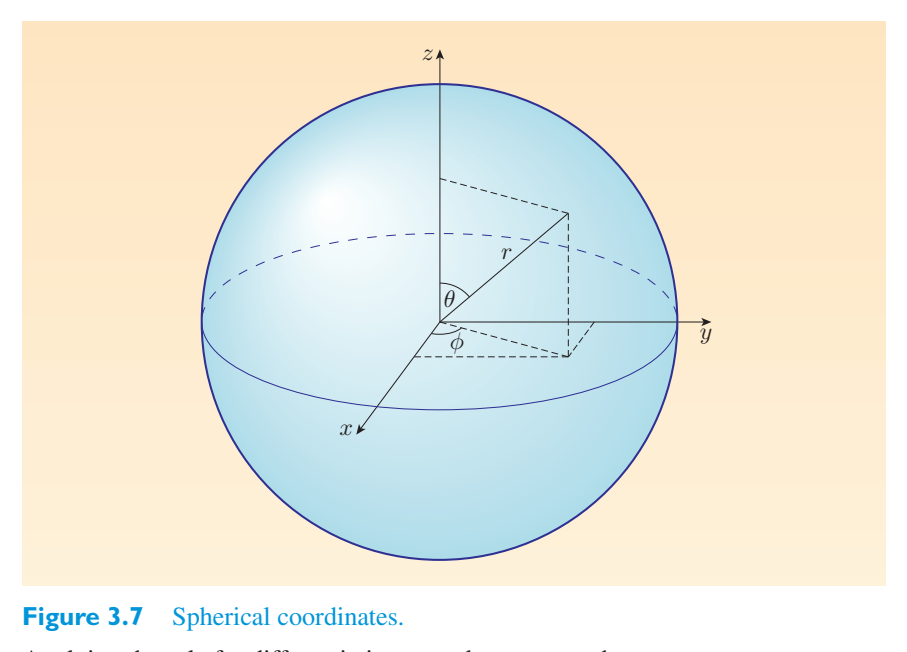
which leads, after some algebra, to经过一些代数运算后,得出
Using these alternative expressions for the line element, we can give meaning to the length of a curve in three-dimensional Euclidean space, and from there we could start to build up the whole of three-dimensional Euclidean geometry, just as we started to do in the two-dimensional case. As Gauss realized, these line elements are really the key to unlocking an entire geometry.使用线元素的这些替代表达式,我们可以赋予三维欧几里德空间中曲线的长度含义,并且从那里我们可以开始构建整个三维欧几里德几何,就像我们在二维情况下开始做的那样。正如高斯意识到的那样,这些线元素确实是解锁整个几何图形的关键。
One topic that we can investigate is the geometry of two-dimensional surfaces in three-dimensional space. If, in Equation 3.9, we set r equal to a constant, R, then we are restricting ourselves to the surface of a sphere of radius R, and the equation for the line element reduces to我们可以研究的主题之一是三维空间中二维表面的几何形状。如果在方程 3.9 中,我们将 r 设置为常数 R,那么我们将自己限制在半径为 R 的球体表面,并且线元素的方程简化为
There are just two variables in Equation 3.10, \(\theta\) and \(\phi\), so it really does describe the geometry of a two-dimensional space. But the geometry of this two-dimensional space — the surface of the sphere — differs significantly from that of the plane, as the following example shows.方程 3.10 中只有两个变量:\(\theta\) 和 \(\phi\),因此它确实描述了二维空间的几何形状。但这个二维空间的几何形状(球体的表面)与平面的几何形状显着不同,如以下示例所示。
Worked Example 3.3工作示例 3.3
Figure 3.8 shows a sphere of radius R and a spherical coordinate system. Suppose that we draw a circle on the sphere by sweeping round the ‘north pole’ at a fixed angle \(\theta\). Starting from Equation 3.10, find the length of the circumference C of the circle.图 3.8 显示了半径为 R 的球体和球坐标系。假设我们以固定角度 \(\theta\) 绕“北极”扫过,在球体上画了一个圆。从公式 3.10 开始,求出圆的周长 C。
Solution解决方案
Since \(\theta\) is constant, Equation 3.10 tells us that a line element along the circle’s circumference is given by \(dl^2\) = \(R^2\) \(\sin^2 \theta\) d \(\phi\) 2. Adding together (i.e. integrating) all the line elements around the circle is easy in this case, since each one points in the direction of increasing \(\theta\), so the circumference is由于 \(\theta\) 是常数,方程 3.10 告诉我们,沿圆圆周的线元由 \(dl^2\) = \(R^2\) \(\sin^2 \theta\) d \(\phi\) 2 给出。在这种情况下,将圆周围的所有线元加在一起(即积分)很容易,因为每个线元都指向 \(\theta\) 增加的方向,因此周长为
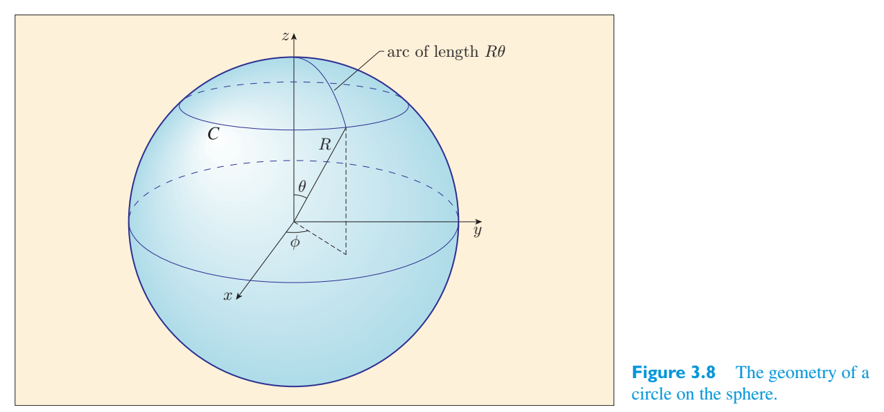
If the geometry of a spherical surface were the same as that of a plane, we would expect the circumference C to be 2 \(\pi\) times the radius of the circle, with both the circumference and the radius measured in the spherical surface. The radius measured in the spherical surface is Rθ, so the geometry of a plane would lead us to expect C = 2 πRθ. However, as the worked example showed, the circumference of the circle on the sphere is actually C = 2 πR sin \(\theta\), which is less than plane geometry implies. So the geometry of a spherical surface is different from that of a plane. This has been well known to mathematicians and navigators for a long time. (Euclid used spherical geometry in his writings on astronomy.) But its real significance was not properly appreciated until the discovery of non-Euclidean geometry (now sometimes called hyperbolic geometry) caused mathematicians to reconsider the nature of geometry in general.如果球面的几何形状与平面的几何形状相同,则我们预计周长 C 为 2 \(\pi\) 乘以圆的半径,并且周长和半径都是在球面中测量的。在球面中测量的半径为 Rθ,因此平面的几何形状将使我们预期 C = 2 πRθ。然而,正如工作示例所示,球体上圆的周长实际上是 C = 2 πR sin \(\theta\),这小于平面几何所暗示的。因此球面的几何形状与平面的几何形状不同。长期以来,这一点已为数学家和航海家所熟知。(欧几里得在他的天文学著作中使用了球面几何。)但直到非欧几里得几何(现在有时称为双曲几何)的发现促使数学家重新考虑一般几何的本质,它的真正意义才得到适当的认识。
We shall not try to formulate spherical geometry here, but it is worth noting some key points that will be of significance later. A topic of great interest in spherical geometry is the behaviour of triangles. Obviously, there are no straight lines on a spherical surface, so before we can discuss spherical triangles, we need to know what are the spherical analogues of straight lines from which such triangles can be constructed. On a spherical surface this special role is played by the arcs of great circles. A great circle is a curve on the surface of a sphere created by the intersection of the sphere and a plane that passes through its centre. (On the Earth, the equator is an example of a great circle, and so are the meridian circles that pass through the North and South Poles.) In a Euclidean plane, the shortest path between any two points is the straight line that joins them. Similarly, on the surface of a sphere, the shortest path between any two points is the minor (i.e. shorter) arc of the great circle that passes through those points.我们不会在这里尝试制定球面几何,但值得注意的是一些稍后将具有重要意义的关键点。球面几何中一个非常有趣的话题是三角形的行为。显然,球面上不存在直线,因此在讨论球面三角形之前,我们需要知道可以构造此类三角形的直线的球面类似物是什么。在球面上,这种特殊的作用是由大圆弧发挥的。大圆是球体表面上的一条曲线,由球体与穿过其中心的平面相交而形成。(在地球上,赤道是大圆的一个例子,穿过北极和南极的子午线圆也是如此。)在欧几里得平面中,任意两点之间的最短路径是联络它们的直线。类似地,在球体表面上,任意两点之间的最短路径是穿过这些点的大圆的短(即较短)弧。
Figure 3.9 shows a spherical triangle constructed from the minor arcs of three great circles. In this case the spherical triangle is a rather special one since each of the interior angles is a right angle, but this illustrates another important difference between spherical geometry and plane geometry: the sum of the interior angles of a spherical triangle is greater than 180 ◦.图 3.9 显示了由三个大圆的短弧构成的球面三角形。在这种情况下,球面三角形是一个相当特殊的三角形,因为每个内角都是直角,但这说明了球面几何与平面几何之间的另一个重要区别:球面三角形的内角之和大于 180°。
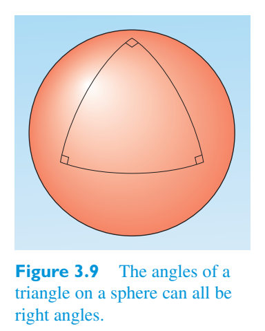
What lies behind the differences between the geometries of a plane and a sphere is the simple fact that the plane is flat while the surface of a sphere is curved. At this stage it is easy to believe that the spherical surface is curved because we can ‘see’ it as a curved two-dimensional surface in a three-dimensional Euclidean space, but this is not generally a reliable guide nor is such visual information always obtainable. Later, a mathematical definition of curvature will be introduced that will confirm the curvature of the spherical surface. However, it’s important to note that we now have two tests for the presence of curvature that do not depend on being able to ‘see’, or even imagine, the curved surface in a space of higher dimension. Using the appropriate two-dimensional line element, we can compare the circumference of a circle with 2 \(\pi\) times the radius, or we can construct a triangle (using paths of shortest length as sides) and compare the sum of the interior angles with 180 ◦. Each of these tests for curvature could be carried out by two-dimensional beings — traditionally called bugs — who live on the two-dimensional surface and have no concept of any higher-dimensional space. From a mathematical point of view this is an indication that curvature is an intrinsic property of a surface that can be determined from measurements made in the surface, rather than an extrinsic property that depends on measurements made in some higher dimension.平面和球体的几何形状差异背后隐藏着一个简单的事实:平面是平坦的,而球体的表面是弯曲的。在这个阶段,很容易相信球面是弯曲的,因为我们可以将其“视为”三维欧几里得空间中的弯曲二维表面,但这通常不是可靠的指导,也并不总是可以获得这样的视觉信息。随后,将引入曲率的数学定义来确认球面的曲率。然而,值得注意的是,我们现在有两个关于曲率存在的测试,这些测试并不依赖于能够“看到”,甚至想象更高维度空间中的曲面。使用适当的二维线元素,我们可以将圆的周长与 2 \(\pi\) 乘以半径进行比较,或者我们可以构造一个三角形(使用最短长度的路径作为边)并将内角和与 180 ° 进行比较。这些曲率测试中的每一个都可以由二维生物(传统上称为虫子)进行,它们生活在二维表面上,没有任何高维空间的概念。从数学的角度来看,这表明曲率是表面的内在属性,可以通过在表面中进行的测量来确定,而不是取决于在某些更高维度中进行的测量的外在属性。
It is important to be aware of the intrinsic nature of curvature and our ability to detect it for at least three reasons. First, unlike spherical surfaces, not all surfaces that are of mathematical interest can be reproduced (the proper term is embedded) in three-dimensional Euclidean space. The ‘hyperbolic’ surface of the original non-Euclidean geometry is of this kind. The geometry exists, but the two-dimensional surface to which it applies cannot be embedded in three-dimensional Euclidean space. Second, when we come to deal with the curvature of the physical four-dimensional spacetime in which we live, it’s very hard to imagine that we might successfully visualize it as existing within some other space or spacetime of even higher dimension. Third, not everything that appears curved in three dimensions really is curved in the mathematical sense. This last point is illustrated by the example of the cylinder given below.出于至少三个原因,了解曲率的内在本质以及我们检测曲率的能力非常重要。首先,与球面不同,并非所有具有数学意义的表面都可以在三维欧几里德空间中再现(嵌入了专有术语)。原始非欧几里得几何的“双曲”曲面就是这种类型。几何体存在,但它所应用的二维表面不能嵌入三维欧几里得空间中。其次,当我们处理我们所生活的物理四维时空的曲率时,很难想象我们可以成功地将其想象为存在于其他更高维度的空间或时空中。第三,并非所有在三维空间中出现弯曲的东西实际上都是数学意义上的弯曲。下面给出的圆柱体示例说明了最后一点。
A cylinder is formed by taking a strip of a plane, say the \(xy\)-plane from x = a to x = b, and rolling it up so that the line x = a becomes identified with the line x = b, as shown in Figure 3.10. Before rolling up the strip, we can draw on it a circle with radius r and circumference 2 πr. We can also draw a triangle whose interior angles add up to 180 ◦. These two features don’t change when we roll up the strip of the plane, so our two-dimensional bugs carrying out local measurements of distances and angles would not be able to detect what we see as extrinsic curvature due to the rolling up in a third dimension. The process of ‘rolling up’ is what enables us to embed the cylindrical surface in three-dimensional space, but it does not produce any intrinsic curvature at all. In fact, the geometry of the cylinder is intrinsically flat.圆柱体是通过取一条平面(例如从 x = a 到 x = b 的 xy 平面)并将其卷起以使线 x = a 与线 x = b 一致而形成的,如图 3.10 所示。在卷起长条之前,我们可以在上面画一个半径为r、周长为2πr的圆。我们还可以画一个内角和为 180° 的三角形。当我们卷起平面条带时,这两个特征不会改变,因此我们进行距离和角度局部测量的二维错误将无法检测到由于在三维中卷起而导致的外在曲率。 “卷起”的过程使我们能够将圆柱表面嵌入三维空间中,但它根本不产生任何内在曲率。事实上,圆柱体的几何形状本质上是平坦的。
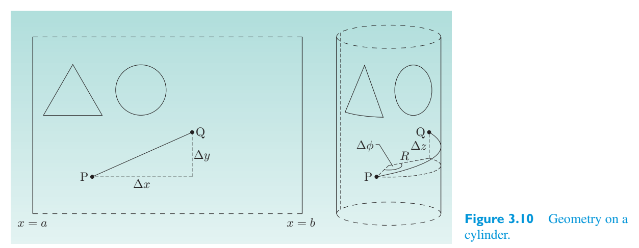
We can approach this idea more mathematically by using the appropriate two-dimensional line elements. The length L of the straight line from P to Q in the plane is given by \(L^{2}\) = (\(\Delta x\)) 2 + (\(\Delta y\)) 2, reminding us that the line element in a plane, expressed in Cartesian coordinates, is \(dl^2\) = \((dx)^2\) + \(dy^2\). Using the cylindrical coordinates (z, \(\phi\)) shown in Figure 3.10, where z is measured parallel to the axis of the cylinder and \(\phi\) is an angle measured in the plane perpendicular to the axis, we see that the distance from P to Q in the cylindrical surface is given by \(L^{2}\) = (\(\Delta z\)) 2 + \(R^2\) (Δ \(\phi\)) 2, where R = (a − b)/2 \(\pi\) is the radius of the cylinder. This shows that the line element in the cylindrical surface will be \(dl^2\) = \(dz^2\) + \(R^2\) d \(\phi\) 2. However, if we make the change of variables x = Rφ, y = z, we see that these two line elements are actually the same.我们可以通过使用适当的二维线元素以更数学的方式来实现这个想法。平面中从 P 到 Q 的直线长度 L 为 \(L^{2}\) = (\(\Delta x\)) 2 + (\(\Delta y\)) 2,这提醒我们平面中的线元以笛卡尔坐标表示为 \(dl^2\) = \((dx)^2\) + \(dy^2\)。使用图 3.10 中所示的圆柱坐标 (z, \(\phi\)),其中 z 是平行于圆柱体轴线测量的,而 \(\phi\) 是在垂直于圆柱体轴线的平面中测量的角度,我们看到圆柱表面中从 P 到 Q 的距离由 \(L^{2}\) = (\(\Delta z\)) 2 + \(R^2\) (Δ \(\phi\)) 2 给出,其中 R = (a − b)/2 \(\pi\) 是圆柱体的半径。这表明圆柱面上的线元将是 \(dl^2\) = \(dz^2\) + \(R^2\) d \(\phi\) 2。但是,如果我们改变变量 x = Rφ,y = z,我们看到这两个线元实际上是相同的。
As a final example of the importance of intrinsic curvature, consider a hotplate consisting of a circular region of the plane with a heat source at the centre point. The heat diffuses through the disc so that it gets cooler as the distance from the heat source increases. The two-dimensional bugs and their measuring sticks expand with the heat, so from our point of view they are bigger towards the centre of the disc (see Figure 3.11), although this is not noticeable to the bugs themselves. As a result of the temperature distribution, the shortest distance from P to Q as measured by the bugs will appear to us to curve in towards the centre, where fewer measuring sticks are needed to cover the distance (this too is shown in Figure 3.11). Hence the angles of the triangle PQR in Figure 3.11 add up to less than 180 ◦, and so, despite looking like a part of a flat plane to us, the hotplate has an intrinsically curved geometry according to the bugs that inhabit it.作为固有曲率重要性的最后一个例子,考虑一个由平面圆形区域组成的加热板,其中心点有一个热源。热量通过圆盘扩散,因此随着与热源距离的增加,圆盘会变得更冷。二维虫子和它们的量尺会随着热量而膨胀,因此从我们的角度来看,它们在靠近圆盘中心的地方会变大(见图 3.11),尽管虫子本身并没有注意到这一点。由于温度分布的原因,虫子测量的从 P 到 Q 的最短距离在我们看来会向中心弯曲,需要更少的测量棒来覆盖该距离(这也如图 3.11 所示)。因此,图 3.11 中三角形 PQR 的角度加起来小于 180°,因此,尽管对我们来说看起来像是平面的一部分,但根据居住在其中的虫子,加热板具有本质上弯曲的几何形状。
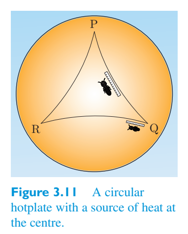
It was Gauss who first recognized the intrinsic nature of the curvature of surfaces, but, as you will see in the next section, it was Riemann who enthusiastically embraced the idea and extended it to spaces of higher dimension.高斯首先认识到曲面曲率的内在本质,但是,正如您将在下一节中看到的那样,黎曼热情地接受了这个想法并将其扩展到更高维度的空间。
Exercise 3.3 Using the same sort of informal arguments练习 3.3 使用相同类型的非正式论证
as in the above examples, investigate the curvature of the following spaces.如上面的示例所示,研究以下空间的曲率。
(a) A cone, excluding the point at its apex. Note that this means that you shouldn’t consider circles and triangles drawn around the apex, as they are not completely contained in the space.(a) 圆锥体,不包括其顶点。请注意,这意味着您不应考虑围绕顶点绘制的圆形和三角形,因为它们并未完全包含在空间中。
(b) A circular ‘hotplate’ where the heat source is around the edge of the disc, so that it cools towards the centre (Figure 3.12).(b) 圆形“加热板”,其中热源位于圆盘边缘周围,以便向中心冷却(图 3.12)。
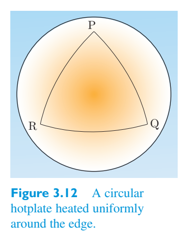
3.2 Metrics and connections3.2 指标和联络
Having informally introduced the idea of a curved space, we now focus on the branch of differential geometry known as Riemannian geometry that is mainly used to analyze such spaces. As we shall see in Chapter 4, it is Riemannian geometry that is particularly relevant to Einstein’s theory of general relativity.在非正式地介绍了弯曲空间的概念之后,我们现在关注微分几何的一个分支,即黎曼几何,它主要用于分析此类空间。正如我们将在第四章中看到的,黎曼几何与爱因斯坦的广义相对论特别相关。
3.2.1 Metrics and Riemannian geometry3.2.1 度规和黎曼几何
In the previous section we saw that in the differential approach to geometry, line elements hold the key to determining lengths of curves and paths of shortest distance, and through them to the properties of circles and triangles, and hence to the whole geometry of Euclidean space or the surface of a sphere. Several line elements were written down for two- and three-dimensional spaces, flat and curved, using a variety of coordinate systems (Equations在上一节中,我们看到,在几何的微分方法中,线元素是确定曲线长度和最短距离路径的关键,并通过它们确定圆和三角形的属性,从而确定欧几里得空间或球体表面的整个几何形状。使用各种坐标系,为二维和三维空间(平面和曲线)写下了几个线元素(方程
3.4, 3.7, 3.8, 3.9,3.4、3.7、3.8、3.9、
3.10). In each case, by analogy with Pythagoras’s theorem,3.10)。在每种情况下,通过与毕达哥拉斯定理类比,
the line element was expressed as a sum of squares of coordinate differentials, such as d x, d y, d r and d \(\theta\). In all those cases the line element was deduced from the known geometrical properties of the space concerned. Riemann’s great insight was to recognize that line elements could be used not merely to summarize a geometry but rather as the starting point for the consideration of a geometry. He realized that by constructing line elements in accordance with certain simple general principles, it would be possible to develop a whole family of geometries that could describe flat and curved spaces with any desired number of dimensions. This is the basis of Riemannian geometry.线元素表示为坐标微分的平方和,例如d x、d y、d r 和d \(\theta\)。在所有这些情况下,线元素都是根据相关空间的已知几何特性推导出来的。黎曼的伟大洞察力是认识到线元素不仅可以用来概括几何,而且可以作为考虑几何的起点。他意识到,通过根据某些简单的一般原理构建线元素,可以开发出一整套几何图形,可以描述具有任何所需维数的平坦和弯曲空间。这是黎曼几何的基础。
An n-dimensional Riemann space is a space in which the line element takes the general formn 维黎曼空间是其中线元素采用一般形式的空间
where d \(x^1\), \((dx)^2\),..., d x n are the differentials of the n coordinates that describe the space, and the various \(g_{ij}\) are functions of the coordinates known as metric coefficients that are required to be symmetric in the sense that \(g_{ij}\) = \(g_{ji}\).其中 d x 1, d x 2,..., d x n 是描述空间的 n 个坐标的微分,各个 \(g_{ij}\) 是被称为度规系数的坐标的函数,这些系数要求在 \(g_{ij}\) = \(g_{ji}\) 的意义上是对称的。
Each of the line elements that we examined in the previous section was a special case of this general Riemannian line element. In the case of the Euclidean plane described by plane polar coordinates, for example, we saw in Equation 3.7 that我们在上一节中研究的每个线单元都是这个一般黎曼线单元的一个特例。例如,在由平面极坐标描述的欧几里得平面的情况下,我们在方程 3.7 中看到:
which corresponds to the choices n = 2, \(x^1\) = r, \(x_{2}\) = \(\phi\) and the metric coefficients g = 1, g = \(r^2\) and g = g = 0.对应于选择 n = 2、\(x^1\) = r、\(x_{2}\) = \(\phi\) 以及度规系数 g = 1、g = \(r^2\) 和 g = g = 0。
In an n-dimensional Euclidean space described by n Cartesian coordinates (\(x^1\), \(x_{2}\), \(x^{3}\),..., x n), the line element is在由 n 个笛卡尔坐标 (x 1, x 2, x 3,..., x n) 描述的 n 维欧几里得空间中,线元素为
and the metric coefficients can be written as \(g_{ij}\) = \(\delta_{ij}\), where \(\delta_{ij}\) is the Kronecker delta defined by度规系数可以写为 \(g_{ij}\) = \(\delta_{ij}\),其中 \(\delta_{ij}\) 是克罗内克增量,定义为
1 if i = j, 0 if \(i\ne j\).如果 i = j,则为 1;如果 \(i\ne j\),则为 0。
In general, the metric coefficients can be regarded as forming an n × n array with \(n^2\) elements, though due to the symmetry requirement \(g_{ij}\) = \(g_{ji}\), the number of independent elements is only n (n + 1)/2, i.e. half the number of off-diagonal elements, plus the n diagonal ones. The complete set of metric coefficients \(g_{\mu\nu}\) is called the metric or sometimes the metric tensor. (We shall not be much concerned with coordinate transformations in this chapter, but you will see later that the metric does transform in the way required of a rank 2 covariant tensor.) Consequently, the metric tensor for the three-dimensional Euclidean space defined by the line element of Equation 3.8 can be written as一般来说,度规系数可以看作是由 \(n^2\) 个元素组成的 n × n 数组,但由于对称性要求 \(g_{ij}\) = \(g_{ji}\),独立元素的数量仅为 n (n + 1)/2,即非对角元素数量加上 n 个对角元素的一半。度规系数 \(g_{\mu\nu}\) 的完整集合称为度规或有时称为度规张量。(本章中我们不会太关心坐标变换,但是稍后您将看到度规确实按照 2 阶协变张量所需的方式进行变换。)因此,由方程 3.8 的线元素定义的三维欧几里得空间的度规张量可以写为
where the i, j simply indicate the positions of the indices and have no other significance. (In much of the literature on general relativity, no explicit distinction is made between a tensor and its components. Rather than follow this potentially confusing practice, we use brackets [] to indicate the full tensor.)其中i、j仅表示索引的位置,没有其他意义。 (在许多关于广义相对论的文献中,张量及其分量之间没有明确的区别。我们不遵循这种可能令人困惑的做法,而是使用括号 [] 来指示完整的张量。)
Note that, in general, the metric coefficients are not constants, but are functions of the coordinates x i. Once the coordinates being used to describe a space have been specified, it is the metric coefficients that perform the crucially important task of relating the coordinate differentials to lengths and thereby determine the geometry of the space. This point is so important to all that follows that it deserves special emphasis. Once you know the metric, the geometry of the space is entirely determined. However, the converse is not true. The geometry does not uniquely determine the metric; this is simply because there are many possible coordinate systems and hence many different ways of writing the metric.注意,一般来说,度规系数不是常数,而是坐标 x i 的函数。一旦指定了用于描述空间的坐标,度规系数就执行将坐标差与长度相关联的至关重要的任务,从而确定空间的几何形状。这一点对于接下来的一切都非常重要,值得特别强调。一旦知道了度规,空间的几何形状就完全确定了。然而,反之则不然。几何形状并不唯一地确定度规;这仅仅是因为有许多可能的坐标系,因此有许多不同的书写度规的方式。
Exercise 3.4 Writing \(x^1\) = \(\theta\), \(x_{2}\) = \(\phi\), find the metric that defines the curved练习 3.4 写出 \(x^1\) = \(\theta\), \(x_{2}\) = \(\phi\),求定义曲线的度规
geometry of the surface of a sphere of radius R with the line element given by Equation 3.10.半径为 R 的球体表面的几何形状,其线元素由公式 3.10 给出。
We have now seen that both flat and curved spaces can be represented by metrics that are diagonal arrays. In fact, diagonal metrics occur whenever we have orthogonal coordinate systems, in which the different sets of grid lines corresponding to the directions of the x i are at right angles to each other. All the coordinate systems that we have used so far, Cartesian, plane polar and spherical, have been of this kind. It turns out that the metrics of interest in general relativity and cosmology are usually orthogonal, so most of the examples of metrics that we use in this book will be diagonal, but non-diagonal arrays are possible.我们现在已经看到,平坦和弯曲的空间都可以用对角数组的度规来表示。事实上,只要我们有正交坐标系,就会出现对角度规,其中与 x i 方向相对应的不同网格线组彼此成直角。迄今为止我们使用过的所有坐标系,笛卡尔坐标系、平面极坐标系和球坐标系,都是这种类型的。事实证明,广义相对论和宇宙学中感兴趣的度规通常是正交的,因此我们在本书中使用的大多数度规示例都是对角的,但非对角数组也是可能的。
Exercise 3.5 Here we consider the metric of three-dimensional练习3.5 这里我们考虑三维的度规
Euclidean space in spherical coordinates. With \(x^1\) = r, \(x_{2}\) = \(\theta\), \(x^{3}\) = \(\phi\), write down the metric coefficients \(g_{ij}\) that correspond to Equation 3.9, i.e.球坐标中的欧几里得空间。令 \(x^1\) = r、\(x_{2}\) = \(\theta\)、\(x^{3}\) = \(\phi\),记下对应于公式 3.9 的度规系数 \(g_{ij}\),即
Exercise 3.6 The metric coefficients for a plane in练习 3.6 中平面的度规系数
polar coordinates have already been given. Rewrite them as an array using appropriate notation.极坐标已经给出。使用适当的符号将它们重写为数组。
Notice that in both of these exercises, the metric is a function of one or more of the coordinates, even though the spaces are certainly flat. This demonstrates that simply observing that the metric is a function of the coordinates is not sufficient to conclude that the space is curved; we may merely have a flat space in a non-Cartesian coordinate system.请注意,在这两个练习中,度规都是一个或多个坐标的函数,即使空间肯定是平坦的。这表明,仅仅观察度规是坐标的函数并不足以得出空间是弯曲的结论;我们可能只是在非笛卡尔坐标系中拥有一个平坦的空间。
We can summarize the main results of this subsection as follows.我们可以将本小节的主要结果总结如下。
Metrics指标
In an n-dimensional Riemann space, the line element is given by在 n 维黎曼空间中,线元素由下式给出
where the \(n^2\) metric coefficients \(g_{ij}\) that define the geometry of the space are symmetric in the sense that \(g_{ij}\) = \(g_{ji}\), and transform as the components of a rank 2 covariant tensor [\(g_{ij}\)] called the metric tensor.其中定义空间几何形状的 \(n^2\) 个度规系数 \(g_{ij}\) 在 \(g_{ij}\) = \(g_{ji}\) 的意义上是对称的,并且变换为称为度规张量的 2 阶协变张量 [\(g_{ij}\)] 的分量。
3.2.2 Connections and parallel transport3.2.2 联络和并行传输
The main purpose of this subsection is to introduce an important set of quantities known as connection coefficients. In an n-dimensional Riemannian space there 1, 2,..., n), though due to are \(n^3\) such coefficients, usually denoted Γ i (i, j, k = symmetry they are not all independent. Despite the indices, the connection coefficients are not the components of a tensor; under a coordinate transformation they do not transform in the way that tensor components must. The connection coefficients are directly related to the metric coefficients and are important in several contexts, including differentiation in curved space and a related process known as parallel transport. We shall start with a physical discussion of parallel transport and then go on to a more mathematical discussion that includes the connection coefficients.本小节的主要目的是介绍一组重要的量,称为联络系数。在 n 维黎曼空间中,有 1, 2,..., n),尽管由于有 \(n^3\) 个这样的系数,通常表示为 Γ i (i, j, k = 对称性,但它们并不都是独立的。尽管有索引,但联络系数并不是张量的组成部分;在坐标变换下,它们不会按照张量分量必须的方式进行变换。联络系数与度规系数直接相关,并且在多种情况下都很重要,包括弯曲空间中的微分和称为并行传输的相关过程。我们将从并行传输的物理讨论开始,然后继续进行包括联络系数在内的更数学的讨论。
Imagine a scientist studying the distribution of wind velocity in the Earth’s atmosphere. The scientist might well want to compare the wind velocity v P at some point P with the wind velocity v Q at some other point Q. To do this, the scientist really needs to convey a copy of v P along some chosen path C to the point Q, preserving the direction of the original v P throughout each infinitesimal step. This is the process of parallel transport. It is illustrated in Figure 3.13, where the copy of v P that has been parallel transported to Q is denoted v # Q.想象一下一位科学家正在研究地球大气层中风速的分布。科学家可能很想将某个点 P 处的风速 v P 与其他点 Q 处的风速 v Q 进行比较。为此,科学家确实需要沿着某个选定的路径 C 将 v P 的副本传送到点 Q,并在每个无穷小步骤中保留原始 v P 的方向。这就是并行传输的过程。如图 3.13 所示,其中已并行传输到 Q 的 v P 的副本表示为 v # Q。
The mathematical difficulty of performing such a parallel transport of a vector along a curve depends very much on the nature of the space and coordinates involved. If the space is Euclidean and the coordinates Cartesian, the process is very simple. The wind velocity at any point can be written as v = v 1 i + \(v^{2}\) j + \(v^{3}\) k, where the unit vectors i, j and k in the \(x^1\) = x, \(x_{2}\) = y and \(x^{3}\) = z directions are said to be coordinate basis vectors, since they point in the direction of increasing coordinate values, and v 1, \(v^{2}\) and \(v^{3}\) are the components of v in the coordinate basis. Since we are using Cartesian coordinates in Euclidean space, a vector may be parallel transported by simply keeping its components constant, so the components of v will be v 1 = v 1, \(v^{2}\) = \(v^{2}\) and \(v^{3}\) = \(v^{3}\).沿着曲线执行矢量的这种平行传输的数学难度很大程度上取决于所涉及的空间和坐标的性质。如果空间是欧几里得坐标,坐标是笛卡尔坐标,则过程非常简单。任意点的风速可以写为 v = v 1 i + \(v^{2}\) j + \(v^{3}\) k,其中 \(x^1\) = x、\(x_{2}\) = y 和 \(x^{3}\) = z 方向上的单位向量 i、j 和 k 被称为坐标基向量,因为它们指向坐标值增加的方向,并且 v 1、\(v^{2}\) 和\(v^{3}\) 是坐标系中 v 的分量。由于我们在欧几里得空间中使用笛卡尔坐标,因此只需保持其分量不变即可并行传输向量,因此 v 的分量将为 v 1 = v 1、\(v^{2}\) = \(v^{2}\) 和 \(v^{3}\) = \(v^{3}\)。
The situation is not so simple if the Cartesian coordinates are replaced by spherical coordinates with \(x^1\) = r, \(x_{2}\) = \(\theta\) and \(x^{3}\) = \(\phi\). The reason for the extra complexity is easy to see and is illustrated in Figure 3.14. Spherical coordinates belong to the family vector along of curvilinear coordinates. That means that the coordinate basis vectors r E, \(\theta\) E and \(\phi\) E change their direction from place to place. As a consequence, in these coordinates, the components of the parallel transported vector at Q, v # Q, will be different from those of the original vector v P at P. So, in order to parallel transport a vector in this case, we need to know exactly how the components must change during each infinitesimal displacement along the curve.如果将笛卡尔坐标替换为球坐标(\(x^1\) = r、\(x_{2}\) = \(\theta\) 和 \(x^{3}\) = \(\phi\)),情况就不那么简单了。额外复杂性的原因很容易看出,如图 3.14 所示。球坐标属于曲线坐标系向量。这意味着坐标基向量 r E、\(\theta\) E 和 \(\phi\) E 的方向会随着位置的不同而改变。因此,在这些坐标中,Q 处的平行传输矢量 v # Q 的分量将不同于 P 处的原始矢量 v P 的分量。因此,为了在这种情况下并行传输矢量,我们需要准确地知道在沿曲线的每个无穷小的位移期间分量必须如何变化。
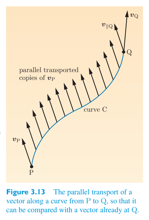
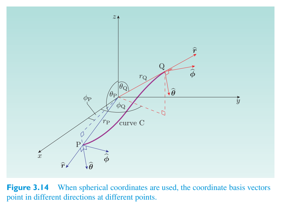
Now let’s generalize this problem to a three-dimensional Riemann space (which may be intrinsically curved) with coordinates \(x^1\), \(x_{2}\), \(x^{3}\) and metric [g] (i, j = 1, 2, 3) in which we want to parallel transport a vector specified at point P along a curve C to point Q. We shall suppose that positions along the curve are described by a parameter u and that the curve is therefore described by three coordinate functions \(x^1\) (u), \(x_{2}\) (u) and \(x^{3}\) (u). If we denote the coordinate basis vectors (the analogues of i, j, k or r E, \(\theta\) E, \(\phi\) E) by e, e, e, then at any point on C that corresponds to the parameter value u, we can write the local value of an arbitrary vector field v(u) in terms of its components in the coordinate basis and the coordinate basis vectors at that point. Thus现在让我们将这个问题推广到一个三维黎曼空间(可能本质上是弯曲的),坐标为 \(x^1\), \(x_{2}\), \(x^{3}\) 和度规 [g] (i, j = 1, 2, 3),其中我们希望将点 P 指定的向量沿着曲线 C 平行传输到点 Q。我们假设沿曲线的位置由参数 u 描述,因此曲线由三个坐标函数 \(x^1\) (u)、\(x_{2}\) (u) 描述和x 3 (u)。如果我们用 e, e, e 表示坐标基向量(i、j、k 或 r E、\(\theta\) E、\(\phi\) E 的类似物),那么在 C 上对应于参数值 u 的任意点,我们可以根据其在坐标基中的分量和该点的坐标基向量来写出任意向量场 v(u) 的局部值。因此
Applying the rule for differentiating a product, we see that the rate of change of the vector field with respect to u as we move along the curve is given by应用对乘积进行微分的规则,我们可以看到,当我们沿着曲线移动时,向量场相对于 u 的变化率由下式给出
where the first term on the right represents the effect of changing the components, while the second term represents the effect of the changing basis vectors. Using the chain rule we can express the last term as a sum of terms, giving其中右侧第一项表示更改分量的影响,而第二项表示更改基向量的影响。使用链式法则,我们可以将最后一项表示为各项之和,给出
Consider the term ∂ e j/∂x k — note that this is a vector quantity. It represents the rate of change of e j with respect to x k and will have components in the direction of each of the basis vectors. This means that we can write it as a sum:考虑术语 ∂ e j/∂x k — 请注意,这是一个向量。它表示 e j 相对于 x k 的变化率,并且具有每个基向量方向上的分量。这意味着我们可以将其写成总和:
where, at any point, \(\Gamma^i{}_{jk}\) represents the component in the direction of basis vector e i of the rate of change of e j with respect to x k. It is the \(n^3\) quantities \(\Gamma^i{}_{jk}\) defined by this equation that are the connection coefficients for the space and coordinates concerned. Since each connection coefficient involves only unit vectors and coordinates, it is clear that it must be determined by the metric; we shall see how a little later.式中,在任意点, \(\Gamma^i{}_{jk}\) 表示 e j 相对于 x k 的变化率在基向量 e i 方向上的分量。该方程定义的 \(n^3\) 个量 \(\Gamma^i{}_{jk}\) 是相关空间和坐标的联络系数。由于每个联络系数只涉及单位向量和坐标,显然必须由度规来确定;我们稍后会看到如何进行。
Substituting Equation 3.14 into Equation 3.13, we see that将公式 3.14 代入公式 3.13,我们可以看到
All of the indices on the right-hand side are summed over, so they are all dummy indices. This means that we can change any of them, provided that we do so consistently. Using this freedom we can rewrite the equation as右侧所有指数都经过求和,因此它们都是虚拟指数。这意味着我们可以改变其中任何一个,只要我们始终如一地这样做。利用这种自由度,我们可以将方程重写为
If we now require that the vector field that we have been discussing represents the same parallel transported vector at every point, then we can say that its rate of change must be zero. So the condition that must be satisfied if the vector v is actually being parallel transported along the curve is that如果我们现在要求我们一直在讨论的向量场在每个点都表示相同的并行传输向量,那么我们可以说它的变化率必须为零。因此,如果向量 v 实际上沿着曲线平行传输,则必须满足的条件是
Thus, even in the case of a curved space, where the geometric interpretation is not simple, we can ensure the parallel transport of a vector by requiring that for each component,因此,即使在几何解释并不简单的弯曲空间的情况下,我们也可以通过要求每个分量确保向量的并行传输,
So, given the components v i (u) of a vector at some point on the curve, the components of the parallel transported vector at a neighbouring point are因此,给定曲线上某个点处向量的分量 v i (u),相邻点处并行传输向量的分量为
All that remains is to determine the expression for the connection coefficient \(\Gamma^i{}_{jk}\) in terms of the metric.剩下的就是确定联络系数 \(\Gamma^i{}_{jk}\) 的度规表达式。
If we consider two nearby points, we can write their infinitesimal vector separation as如果我们考虑两个附近的点,我们可以将它们的无穷小向量间隔写为
and consequently因此
Comparing this with the original line element (Equation 3.11)将其与原始线元素进行比较(公式 3.11)
we see that我们看到
So the basis vectors are directly related to the metric coefficients.因此基向量与度规系数直接相关。
Now, if we partially differentiate Equation 3.20 with respect to x k, we see that现在,如果我们对方程 3.20 对 x k 进行部分微分,我们会看到
Using Equation 3.14 again, this can be rewritten as再次使用公式 3.14,可以将其重写为
After several lines of additional algebra, this leads to the final result经过几行附加代数后,得出最终结果
metric tensor [\(g_{ij}\)]. This where g il is a component of the contravariant form of the that is, [\(g_{ij}\)][\(g_{ij}\)] is equal latter quantity is the inverse of [\(g_{ij}\)] regarded as a matrix; to the identity matrix or, more explicitly,度规张量 [\(g_{ij}\)]。其中 g il 是的逆变形式的一个分量,即 [\(g_{ij}\)][\(g_{ij}\)] 等于后一个量,是被视为矩阵的 [\(g_{ij}\)] 的逆;到单位矩阵,或者更明确地说,
Since [\(g_{ij}\)] is the inverse of the metric [\(g_{ij}\)], it too must contain all the information about the geometry of the space. It is sometimes referred to as the dual metric.由于 [\(g_{ij}\)] 是度规 [\(g_{ij}\)] 的倒数,因此它也必须包含有关空间几何形状的所有信息。它有时被称为双度规。
Our findings regarding parallel transport can now be summarized as follows.我们关于并行传输的发现现在可以总结如下。
Parallel transport and connection coefficients并行传输和联络系数
Given the components v i of a vector at some point on a curve specified by x i (u) in a Riemann space with coordinates x i,..., x n and metric [g], the components of the parallel transported vector at some neighbouring point on the curve are given by给定在坐标 x i,..., x n 和度规 [g] 的黎曼空间中由 x i (u) 指定的曲线上某个点处向量的分量 v i,曲线上某个相邻点处的平行传输向量的分量由下式给出
where the connection coefficient \(\Gamma^i{}_{jk}\) is given by其中联络系数 \(\Gamma^i{}_{jk}\) 由下式给出
and the dual metric [\(g_{ij}\)], the matrix inverse of [\(g_{ij}\)], is defined by the requirement that对偶度规 [\(g_{ij}\)]([\(g_{ij}\)] 的矩阵逆)由以下要求定义:
i jk for:我想:
Exercise 3.7 Calculate the connection coefficients Γ练习 3.7 计算联络系数 Γ
(a) a two-dimensional Euclidean space using Cartesian coordinates; (b) the surface of a sphere of radius R = 1, using polar coordinates.(a) 使用笛卡尔坐标的二维欧几里得空间; (b) 半径 R = 1 的球体表面,使用极坐标。
As mentioned earlier, connection coefficients and parallel transport are important in several contexts, particularly in connection with differentiation in curved spaces. However, as Exercise 3.7 shows, they also provide an important indicator of the curvature of a space. Two-dimensional surfaces provide some easily visualized examples of this. In the case of the cylinder shown in Figure 3.15, parallel transport does exactly what it says: if we transport a vector v around a closed curve, it stays parallel to itself all the way around and gets back to the initial point exactly as it started out. That’s because the surface of a cylinder is actually a flat space in terms of its intrinsic geometry.如前所述,联络系数和平行传输在多种情况下都很重要,特别是与弯曲空间的微分相关。然而,正如练习 3.7 所示,它们还提供了空间曲率的重要指标。二维表面提供了一些易于可视化的示例。在图 3.15 所示的圆柱体中,平行传输的作用正如其所言:如果我们绕一条闭合曲线传输一个向量 v,它自始至终都保持与自身平行,并准确地回到起始点。这是因为,就其内在几何形状而言,圆柱体的表面实际上是一个平坦的空间。
However, as shown in Figure 3.16, there are no parallel lines in the curved geometry of a spherical surface, so we can’t really expect that even a vector that is parallel transported over infinitesimal steps will manage to stay ‘parallel’ to itself when transported around a loop of finite size. And indeed, after being moved around a closed spherical triangle by ‘parallel’ transport, the vector in Figure 3.16 arrives back at its starting position pointing in a different direction.然而,如图 3.16 所示,球面的弯曲几何形状中不存在平行线,因此我们不能真正期望即使是在无穷小的步长上平行传输的向量,在绕有限大小的环传输时也能设法保持与其自身“平行”。事实上,在通过“平行”传输围绕闭合球形三角形移动后,图 3.16 中的矢量返回到指向不同方向的起始位置。
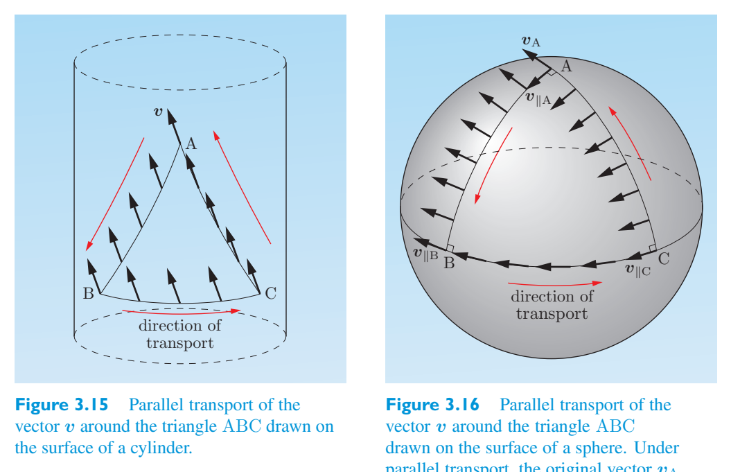
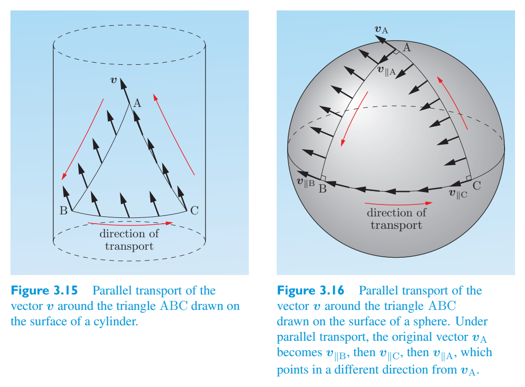
vector v around the triangle ABC drawn on the surface of a cylinder.围绕在圆柱体表面绘制的三角形 ABC 的矢量 v。
Thus parallel transport of a vector around a closed curve or path gives us another test for whether a particular geometry is intrinsically flat or curved. Indeed, as you will see later, the difference between the initial and final directions of the vector gives us a measure of just how curved the geometry is in the vicinity of the closed path.因此,矢量围绕闭合曲线或路径的平行传输为我们提供了另一种测试,以确定特定几何形状本质上是平坦的还是弯曲的。事实上,正如您稍后将看到的,矢量的初始方向和最终方向之间的差异使我们能够衡量闭合路径附近几何形状的弯曲程度。
3.3 Geodesics3.3 测地线
In a flat space, straight lines are of particular importance. A straight line represents the most direct route between two points and also the path of shortest distance between those points. Great circles play a similar role in the curved surface of a sphere. The analogues of straight lines and great circles in a general Riemannian space are referred to as geodesics. In this section we generalize the notions of ‘most direct path’ and ‘shortest distance’ in order to present two different derivations of the equations that are used to determine geodesics.在平坦的空间中,直线尤为重要。直线代表两点之间最直接的路线,也是两点之间距离最短的路径。大圆在球体的曲面中起着类似的作用。一般黎曼空间中直线和大圆的类似物被称为测地线。在本节中,我们概括了“最直接路径”和“最短距离”的概念,以呈现用于确定测地线的方程的两种不同推导。
3.3.1 Most direct route between two points3.3.1 两点之间最直接的路线
One way of defining a straight line in Euclidean space is as a curve that always goes in the same direction. In order to extend this definition to the more general spaces of Riemannian geometry, we need to analyze the concept of ‘direction along a curve’ and what it means to ‘always go in the same direction’. At any coordinate functions x i (u) point on a curve parameterized by u and defined by the (i = 1,..., n), we can define the tangent vector t to be the vector that points along the curve, as shown in Figure 3.17. The components of such a vector are t i = d x i/d u. If the curve is always going to go in the same direction, then the tangent vector should not change its direction as the parameter u varies and the tangent vector travels along the curve. In other words, if we parallel transport the by u + d u, the resulting tangent vector at u along the curve C to the point specified vector should be proportional to the tangent vector at u在欧几里得空间中定义直线的一种方法是定义为始终沿同一方向行进的曲线。为了将这个定义扩展到黎曼几何的更一般空间,我们需要分析“沿曲线的方向”的概念以及“始终沿同一方向行进”的含义。在由 u 参数化并由 (i = 1,..., n) 定义的曲线上的任意坐标函数 x i (u) 点,我们可以将切向量 t 定义为沿曲线指向的向量,如图 3.17 所示。该向量的分量为 t i = d x i/d u。如果曲线始终沿同一方向行进,则切向量不应随着参数 u 的变化而改变其方向,并且切向量沿曲线行进。换句话说,如果我们通过 u + d u 平行传输,则沿曲线 C 到点指定向量在 u 处得到的切向量应该与 u 处的切向量成正比
where f (u) is some function of u. It then follows from the condition for parallel transport that for each component of t,其中 f (u) 是 u 的某个函数。然后根据并行传输的条件得出对于 t 的每个分量,
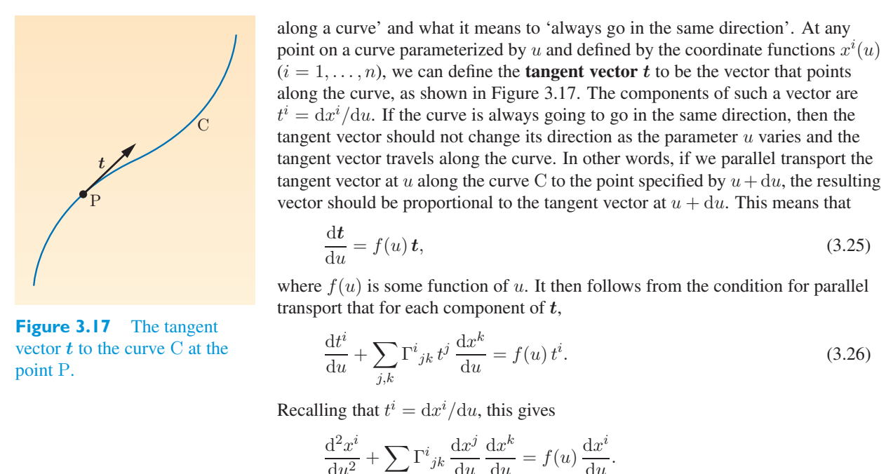
Recalling that t i = d x i/d u, this gives回想一下 t i = d x i/d u,这给出
Now this can be simplified by choosing the parameter u in such a way that the function f (u) is equal to zero. When the parameter is chosen in this particular way, it is said to be an affine parameter and will be denoted by the symbol \(\lambda\). (This choice ensures that the tangent vector will preserve its magnitude as well as its direction as we move along the curve.) So, provided that we choose to use an affine parameter \(\lambda\), the condition for a parameterized curve defined by a set of coordinate functions x i (\(\lambda\)) to always point in the same direction is that现在可以通过选择参数 u 使函数 f (u) 等于 0 来简化。当以这种特定方式选择参数时,它被称为仿射参数,并用符号 \(\lambda\) 表示。(此选择确保当我们沿着曲线移动时,切向量将保留其大小和方向。)因此,假设我们选择使用仿射参数 \(\lambda\),则由一组坐标函数 x i (\(\lambda\)) 定义的参数化曲线始终指向同一方向的条件是:
These are called the geodesic equations. Any parameterized pathway defined by a set of n functions x i (\(\lambda\)), i = 1,..., n, that satisfies these differential equations is said to be a geodesic in the n-dimensional Riemannian space with metric [\(g_{ij}\)] and connection coefficients \(\Gamma^i{}_{jk}\). This is the analogue of a straight line in the curved space.这些称为测地线方程。任何由一组 n 个函数 x i (\(\lambda\)), i = 1,..., n 定义且满足这些微分方程的参数化路径被称为 n 维黎曼空间中的测地线,其度规为 [\(g_{ij}\)] 和联络系数 \(\Gamma^i{}_{jk}\)。这类似于弯曲空间中的直线。
3.3.2 Shortest distance between two points3.3.2 两点之间的最短距离
We saw earlier that in a two-dimensional Euclidean space, the length of a curve, and y (u), between the parameterized by u and defined by the functions x (u) d l from P to Q points P and Q is given by integrating the line element (Equation 3.6) so that我们之前看到,在二维欧几里得空间中,曲线的长度和 y (u)(由 u 参数化并由函数 x (u) d l 定义,从 P 到 Q 点 P 和 Q 是通过对线元素进行积分而给出(方程 3.6),因此
In an n-dimensional Riemannian space, Equation 3.11 extends the definition of the line element to include the metric via在 n 维黎曼空间中,方程 3.11 扩展了线元素的定义以包括度规通过
so we must correspondingly extend the formula for the length of the curve to所以我们必须相应地将曲线长度的公式推广为
What we want to find is the parameterized curve (\(x^1\) (u), \(x_{2}\) (u),..., x n (u)) between P and Q that gives the smallest value for L (P, Q), i.e. the shortest distance between the two points. Such a curve would be the analogue of a straight line, and therefore a geodesic. We use a method that is analogous to finding the minimum of a function f (x) by differentiating it and looking for points at which d f/d x = 0. The full mathematical treatment uses the calculus of variations, which is beyond the scope of this book, although a flavour of it is sketched below. You are not expected to follow the details, unless you have prior knowledge of the calculus of variations.我们想要找到的是 P 和 Q 之间的参数化曲线 (\(x^1\) (u), \(x_{2}\) (u),..., x n (u)),它给出 L (P, Q) 的最小值,即两点之间的最短距离。这样的曲线类似于直线,因此是测地线。我们使用的方法类似于通过对函数 f (x) 求导并寻找 d f/d x = 0 处的点来查找函数 f (x) 的最小值。完整的数学处理使用了变分法,这超出了本书的范围,尽管下面概述了它的一些风格。除非您事先了解变分法,否则您不需要遵循细节。
We can see from Figure 3.18 that since the geodesic between P and Q is the path of shortest length L, the curves that are close to it are of almost the same length. Now, if we consider all possible curves linking P and Q, and in each case we imagine changing the curve very slightly by making an infinitesimal variation of the form x i (u) → x i (u) + δx i (u), then in each case the length of the curve will change by a small amount δL. However, in the case of the true geodesic, where the length is a minimum, we will find that δL is zero. So, writing从图3.18中我们可以看出,由于P和Q之间的测地线是最短长度L的路径,因此靠近它的曲线的长度几乎相同。现在,如果我们考虑联络 P 和 Q 的所有可能的曲线,并且在每种情况下,我们想象通过进行 x i (u) → x i (u) + δx i (u) 形式的无穷小变化来非常轻微地改变曲线,那么在每种情况下,曲线的长度都会改变少量 δL。然而,在真正的测地线的情况下,长度最小,我们会发现 δL 为零。所以,写
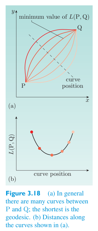
it can be shown that可以证明
Integrating the second part of the sum by parts, and noting that将总和的第二部分按部分积分,并注意到
leads to导致
However, δx m = 0 at P and Q for all m, so the first bracket is zero. Consequently, for δL = 0, we have然而,对于所有 m,在 P 和 Q 处 δx m = 0,因此第一个括号为零。因此,对于 δL = 0,我们有
Since this is true for arbitrary variation δx m, we obtain由于对于任意变化 δx m 都是如此,我们得到
These are known as the Euler–Lagrange equations and are of fundamental importance to the study of the calculus of variations. If we substitute the expression for F(Equation 3.29) into the Euler–Lagrange equations, and choose u so that it is an affine parameter \(\lambda\), it can be shown that这些方程被称为欧拉-拉格朗日方程,对于变分法的研究至关重要。如果我们将 F(方程 3.29)的表达式代入欧拉-拉格朗日方程,并选择 u 使其成为仿射参数 \(\lambda\),则可以证明:
These are just the geodesic equations again (Equation 3.27), which shows that both methods of generalizing the definition of a straight line lead to the same concept of the geodesic.这些又只是测地线方程(方程 3.27),这表明两种推广直线定义的方法都得出相同的测地线概念。
So, to summarize, we have the following.因此,总而言之,我们有以下内容。
Geodesics and the geodesic equations测地线和测地线方程
In an n-dimensional Riemannian space, the analogues of straight lines are known as geodesics. A geodesic can be represented by a curve parameterized by an affine parameter \(\lambda\) and defined by a set of n coordinate functions x i (\(\lambda\)) that satisfy the geodesic equations在 n 维黎曼空间中,直线的类似物称为测地线。测地线可以用一条曲线表示,该曲线由仿射参数 \(\lambda\) 参数化,并由满足测地线方程的一组 n 个坐标函数 x i (\(\lambda\)) 定义
Exercise 3.8 Solve the geodesic equations for two-dimensional练习 3.8 求解二维测地线方程
Euclidean space and verify that the geodesics are indeed straight lines.欧几里得空间并验证测地线确实是直线。
Exercise 3.9 Figure 3.19 shows three curves on the练习 3.9 图 3.19 显示了 3 条曲线
surface of a sphere:球体表面:
- • a portion of a meridian A, with end-points (\(\pi\), 0) and• 子午线 A 的一部分,其端点为 (\(\pi\), 0) 和
- • the equator B, defined by \(\theta\) = \(\pi\) and 0 ≤ \(\phi\) < 2 \(\pi\)赤道 B,定义为 \(\theta\) = \(\pi\) 且 0 ≤ \(\phi\) < 2 \(\pi\)
- • a line of latitude C, defined by \(\theta\) = \(\pi\) and 0 ≤ \(\phi\) < 2• 一条纬度线 C,定义为 \(\theta\) = \(\pi\) 且 0 ≤ \(\phi\) < 2
\(\pi\).\(\pi\)。
Starting from the geodesic equations (Equation 3.27), show that for the curves A, B and C in Figure 3.19:从测地线方程(方程 3.27)开始,显示对于图 3.19 中的曲线 A、B 和 C:
(a) curve A is a geodesic;(a) 曲线A是测地线;
(b) curve B is also a geodesic;(b) 曲线B也是测地线;
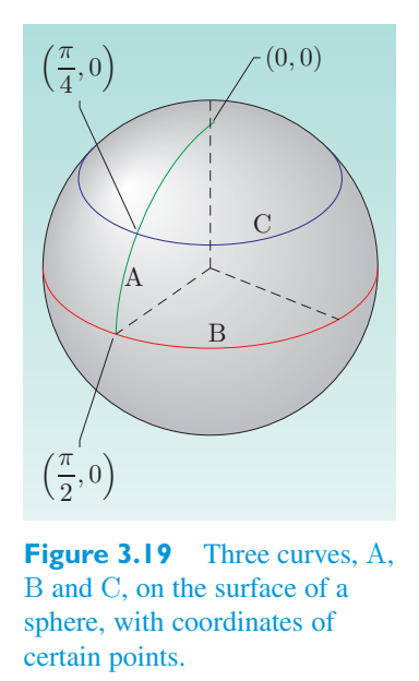
(c) the line of latitude C is not a geodesic.(c) 纬线 C 不是测地线。
3.4 Curvature3.4 曲率
In this section we formalize and quantify the notion of the curvature of space. In particular we learn how to measure the curvature in an intrinsic way that does not depend on being able to embed the space being studied in some other space of higher dimension.在本节中,我们形式化并量化了空间曲率的概念。特别是,我们学习如何以内在的方式测量曲率,而不依赖于能够将正在研究的空间嵌入到其他更高维度的空间中。
3.4.1 Curvature of a curve in a plane3.4.1 平面内曲线的曲率
We start with the comparatively simple idea of a curved line in a plane. Looking at the curve AH in Figure 3.20, it makes sense to say that the section around BCD is ‘more curved’ than the section around EFG. Our first objective is to associate a quantity k with this curvature at each point, such that k C > k F.我们从平面中的曲线这一相对简单的想法开始。观察图 3.20 中的曲线 AH,可以说 BCD 周围的部分比 EFG 周围的部分“更弯曲”。我们的第一个目标是将量 k 与每个点的曲率相关联,使得 k C > k F。
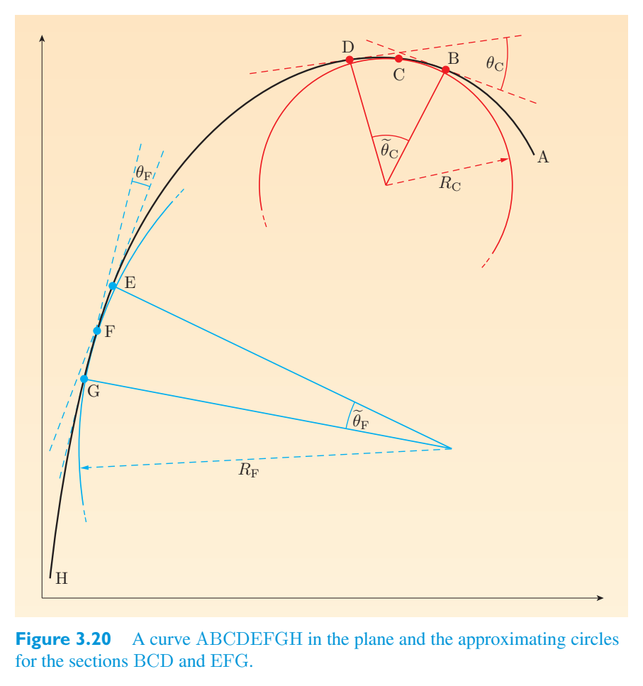
and as l gets smaller, the approximations get better. We can do the same thing with the section EFG of the curve, also of length l, although this time the angle \(\theta\) F between the tangents is smaller than \(\theta\) C, and the radius R F of the approximating circle is larger than R C. This gives the relation随着 l 变小,近似值变得更好。我们可以对曲线的截面 EFG 做同样的事情,长度也是 l,尽管这次切线之间的角度 \(\theta\) F 小于 \(\theta\) C,并且近似圆的半径 R F 大于 R C。这给出了关系
Using the angles between the tangents as the measure of curvature, we can say that使用切线之间的角度作为曲率的度规,我们可以说
curvature at C > curvature at FC 处的曲率 > F 处的曲率
because因为
But但
and \(\theta\) ≈和 \(\theta\) ≈
so所以
and therefore因此
Consequently, the quantity因此,数量
is a measure of the curvature at any point X of a curve C in the plane, where R X is the radius of the circle that best approximates C in the region close to X.是平面中曲线 C 的任意点 X 处曲率的度规,其中 R X 是靠近 X 的区域中最接近 C 的圆的半径。
\(k = 0\).2 c\(\mathrm{m^{-1}}\)?\(k = 0\).2 厘米 - 1?
Exercise 3.10 (a) What is the curve of constant curvature练习 3.10 (a) 什么是常曲率曲线
(b) What is the curvature k = 1/R of a straight line?(b) 直线的曲率 k = 1/R 是多少?
For more complicated curves, a better way of finding the radius of the approximating circle is needed. It can be shown that if a curve is parameterized by the coordinate functions (x (\(\lambda\)), y (\(\lambda\))), then its curvature对于更复杂的曲线,需要更好的方法来找到近似圆的半径。可以证明,如果一条曲线由坐标函数 (x (\(\lambda\)), y (\(\lambda\))) 参数化,那么它的曲率
where a single dot over a function indicates the first derivative of that function with respect to \(\lambda\), and a double dot indicates the second derivative.其中函数上的单点表示该函数相对于 \(\lambda\) 的一阶导数,双点表示二阶导数。
\(x_{2}\) at x = 0. Where is\(x_{2}\) 在 x = 0 处。其中
Exercise 3.11 Find the curvature of the parabola y =练习 3.11 求抛物线的曲率 y =
the centre of the circle that best approximates the parabola in the region close to x = 0?在接近 x = 0 的区域中最接近抛物线的圆心?
Exercise 3.12 Find the curvature at any point on an练习 3.12 求曲线上任意点的曲率
ellipse parameterized by x = a cos \(\lambda\), y = b sin \(\lambda\). Use your answer to show that it leads to the expected result for the curvature of a circle of radius R.椭圆由 x = a cos \(\lambda\)、y = b sin \(\lambda\) 参数化。使用你的答案来证明它可以得出半径为 R 的圆的曲率的预期结果。
3.4.2 Gaussian curvature of a two-dimensional3.4.2 二维的高斯曲率
surface表面
We now consider the curvature of a two-dimensional surface embedded in three-dimensional Euclidean space. Suppose that we want to measure the curvature at a point A on the two-dimensional surface. From the point of view of the three-dimensional space, we can construct a vector N, normal to the surface at A, and this partly defines a plane PL containing N. As shown in Figure 3.21, the plane intersects the two-dimensional surface to give a curve C. (If we fix the two end-points of C in the plane PL, then the curve C is in fact a geodesic.) The curvature of C can be measured, as in the previous subsection, by finding the circle that best approximates the curve at A and then taking the reciprocal of the radius of that circle to obtain the curvature k. However, the plane PL is not completely defined since it can have any orientation with respect to N: different orientations will give different curves C and hence different curvatures k. We can get a measure of the curvature of the two-dimensional surface (rather than just a single curve C) at A by letting the plane PL rotate about N and picking the largest and smallest values of k, which we can denote by k max and k min. The curvature of the two-dimensional surface at A is then characterized by what is known as the Gaussian curvature, which is defined by我们现在考虑嵌入三维欧几里得空间中的二维表面的曲率。假设我们要测量二维表面上 A 点的曲率。从三维空间的角度来看,我们可以构造一个向量N,垂直于A处的曲面,这部分定义了包含N的平面PL。如图3.21所示,该平面与二维曲面相交得到曲线C。(如果我们将 C 的两个端点固定在平面 PL 上,则曲线 C 实际上是测地线。)如上一小节所述,可以通过找到最接近 A 处曲线的圆来测量 C 的曲率,然后取该圆的半径的倒数以获得曲率 k。然而,平面 PL 并未完全定义,因为它可以具有相对于 N 的任何方向:不同的方向将给出不同的曲线 C,从而给出不同的曲率 k。通过让平面 PL 绕 N 旋转并选取 k 的最大和最小值(我们可以用 k max 和 k min 表示),我们可以测量 A 处二维表面(而不仅仅是一条曲线 C)的曲率。然后,A 处二维表面的曲率用所谓的高斯曲率来表征,其定义为
is the intersection between One important subtlety is that for different curves at the same point A on a the surface and the plane PL surface, the approximating circles may lie on opposite sides of the surface: for through N. instance, this occurs in Figure 3.22(a) but not in Figure 3.22(b). In order to distinguish between these situations, we define the curvature k to be positive if the centre of the approximating circle is on the opposite side to the arrowhead of the normal vector N, and negative if it is on the same side. To ensure a unique result, negative curvatures are always taken as being smaller than positive ones in the search for k max and k min. (Of course, the orientation of N is arbitrary, but this doesn’t matter.)一个重要的微妙之处是,对于曲面和平面 PL 曲面上同一点 A 处的不同曲线,近似圆可能位于曲面的相对两侧:对于通过 N 的实例,这种情况出现在图 3.22(a) 中,但不在图 3.22(b) 中。为了区分这些情况,如果近似圆的中心与法向量N的箭头相反一侧,我们定义曲率k为正,如果在同一侧,则曲率k为负。为了确保结果唯一,在搜索 k max 和 k min 时始终将负曲率视为小于正曲率。 (当然,N的方向是任意的,但这并不重要。)
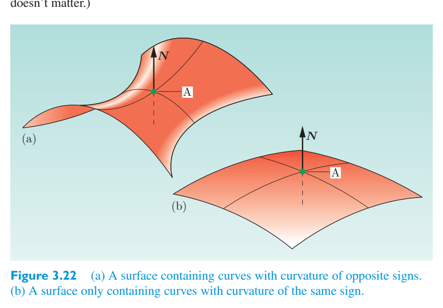
- ● What is the Gaussian curvature for the surface of a two-dimensional sphere of二维球体表面的高斯曲率是多少
radius R?半径R?
❍ For the sphere,❍ 对于球体,
so the Gaussian curvature is所以高斯曲率是
So far, our arguments have depended on being able to embed the surface being studied in a three-dimensional space so that it has an obvious extrinsic curvature. In 1828 Gauss discovered a result regarding the curvature of surfaces that surprised him so much that he called it the ‘remarkable theorem’ (theorema egregium). The theorem provided a formula for working out the Gaussian curvature K of a two-dimensional surface, but the remarkable aspect of the result was that it showed K to be an invariant, independent of the coordinate system used. This was one of the inspirations for Riemann’s work, and is now seen as an indication that curvature is an intrinsic property; it can be calculated directly from the metric [\(g_{ij}\)] and does not require any embedding in a space of higher dimension. We shall not prove the theorema egregium here — even an outline proof requires four pages of dense mathematics — but we shall return to its main outcome once we have considered the curvature of spaces with three or more dimensions, in the next subsection.到目前为止,我们的论点依赖于能够将所研究的表面嵌入到三维空间中,使其具有明显的外在曲率。 1828 年,高斯发现了一个关于曲面曲率的结果,这让他非常惊讶,以至于他将其称为“非凡定理”(theorema egregium)。该定理提供了计算二维表面高斯曲率 K 的公式,但结果的显着之处在于它表明 K 是一个不变量,与所使用的坐标系无关。这是黎曼工作的灵感之一,现在被视为曲率是一种内在属性的迹象;它可以直接从度规 [\(g_{ij}\)] 计算出来,不需要在更高维度的空间中进行任何嵌入。我们不会在这里证明这个定理——即使是一个大纲证明也需要四页的密集数学——但是一旦我们在下一小节中考虑了具有三个或更多维度的空间的曲率,我们将回到它的主要结果。
3.4.3 Curvature in spaces of higher dimensions3.4.3 高维空间中的曲率
Now consider an n-dimensional Riemann space with metric [\(g_{ij}\)] that can be used = 1,..., n). Suppose that to determine the space’s connection coefficients Γ i (i we have a vector v specified at some point P and that we parallel transport that specified by d x j vector around an infinitesimal rectangle PQRS with sides and d x k. This process is illustrated in Figure 3.23, where the parallel transported vector that arrives back at P is denoted v # P and is shown as being different from v because of the curvature of the space. We should expect the difference现在考虑一个 n 维黎曼空间,其度规 [\(g_{ij}\)] 可以使用 = 1,..., n)。假设为了确定空间的联络系数 Γ i (i,我们在某个点 P 处指定了一个向量 v,并且我们将由 d x j 向量指定的向量围绕一个边长为 d x k 的无穷小矩形 PQRS 进行并行传输。这个过程如图 3.23 所示,其中返回 P 的并行传输向量表示为 v # P,并且由于空间的曲率而显示为与 v 不同。我们应该期待差异
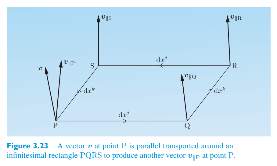
v # P at point P.v # P 在 P 点。
between v # P and v to have components that are proportional to the infinitesimal displacements and to the components of the original vector, so we can write any given component of the difference asv # P 和 v 之间的分量与无穷小位移和原始向量的分量成比例,因此我们可以将差值的任何给定分量写为
where \(R^l{}_{ijk}\) will be some measure of the curvature. (In a flat space we know that v # P = v, so in that case we know that \(R^l{}_{ijk}\) = 0 for all choices of i, j, k and l.) When the parallel transport is actually carried out, it can be shown that其中 \(R^l{}_{ijk}\) 是曲率的某种度规。 (在平坦空间中,我们知道 v # P = v,因此在这种情况下,我们知道对于 i、j、k 和 l 的所有选择,\(R^l{}_{ijk}\) = 0。)当并行传输实际进行时,可以证明:
It turns out that under a general coordinate transformation, the quantity \(R^l{}_{ijk}\) transforms in the manner required of a rank 4 tensor with one contravariant index and three covariant indices. Consequently, \(R^l{}_{ijk}\) is known as the Riemann curvature tensor or the Riemann tensor. It is possible to show that the vanishing of the Riemann tensor [\(R^l{}_{ijk}\)] at all points in a space is a necessary and sufficient condition for a space to be flat, i.e. not curved. So we finally have a quantitative measure of curvature, and — since it is related directly to the metric, albeit in a complicated way — it is clearly an intrinsic quantity that does not require any embedding in higher dimensions.事实证明,在一般坐标变换下,量 \(R^l{}_{ijk}\) 按照具有一个逆变索引和三个协变索引的 4 阶张量所需的方式进行变换。因此,\(R^l{}_{ijk}\) 被称为黎曼曲率张量或黎曼张量。可以证明,空间中所有点的黎曼张量[\(R^l{}_{ijk}\)]消失是空间平坦的充要条件,即不弯曲。因此,我们最终有了曲率的定量测量,而且——因为它与度规直接相关,尽管方式很复杂——它显然是一个内在的量,不需要任何更高维度的嵌入。
In n dimensions the Riemann tensor has \(n^4\) components, giving \(2^4=16\) components in two dimensions and \(3^4=81\) in three dimensions. However, because of the definition of the connection (Equation 3.23) and Equation 3.35 itself, the Riemann tensor has many symmetries involving its indices. For example,在 n 维中,黎曼张量有 \(n^4\) 个分量,在二维中给出 \(2^4=16\) 个分量,在三维中给出 \(3^4=81\) 个分量。然而,由于联络的定义(方程 3.23)和方程 3.35 本身,黎曼张量具有许多涉及其索引的对称性。例如,
These symmetries reduce the number of in dependent components to 6 in three-dimensional spaces and only one in two-dimensional spaces. In two dimensions, the single independent component can be related to the Gaussian curvature K. From the point of view of Riemannian geometry, this is the explanation of Gauss’s theorema egregium, with its implication that Gaussian curvature is intrinsic.这些对称性将三维空间中独立分量的数量减少到 6 个,而在二维空间中仅减少一个。在二维中,单个独立分量可以与高斯曲率K联系起来。从黎曼几何的角度来看,这就是高斯定理egregium的解释,意味着高斯曲率是内在的。
Exercise 3.13 Use Equation 3.35 to show that R l = − R l.练习 3.13 使用方程 3.35 证明 R l = − R l。
Exercise 3.14 Find the Riemann tensor for two-dimensional Euclidean练习 3.14 求二维欧几里得的黎曼张量
space with the line element given by Equation 3.4. Extend your result to an n-dimensional Euclidean space. (Hint: Use Equation 3.35 and the results of Exercise 3.7(a).)空间与方程 3.4 给出的线元素。将结果扩展到 n 维欧几里得空间。 (提示:使用公式 3.35 和练习 3.7(a) 的结果。)
Exercise 3.15 Find the component \(R^{1}\) 212 of the Riemann tensor for a练习 3.15 求黎曼张量的分量 \(R^1{}_{212}\)
two-dimensional sphere of radius R with the line element given in Equation 3.10. (Hint: Use Equation 3.35 and the results of Exercise 3.7(b).)半径为 R 的二维球体,其线元素如公式 3.10 所示。 (提示:使用公式 3.35 和练习 3.7(b) 的结果。)
Exercise 3.16 The Gaussian curvature K for a two-dimensional surface is练习3.16 二维表面的高斯曲率K为
related to the Riemann tensor by where与黎曼张量相关,其中
and the first index of R 1212 is ‘lowered’ by means of the metric tensor (see Chapter 2). Use the result of the earlier in-text question concerning the Gaussian curvature for the surface of a two-dimensional sphere and the results of Exercises 3.7 and 3.15 to verify this relationship for a two-dimensional sphere of radius a. (We use a for the radius of the sphere in order to avoid possible confusion with the Riemann tensor.)R 1212 的第一个索引通过度规张量“降低”(参见第 2 章)。使用先前有关二维球体表面高斯曲率的文内问题的结果以及练习 3.7 和 3.15 的结果来验证半径为 a 的二维球体的这种关系。 (我们使用 a 表示球体的半径,以避免与黎曼张量混淆。)
So, to summarize, we have the following.因此,总而言之,我们有以下内容。
The Riemann tensor黎曼张量
In an n-dimensional Riemannian space, the curvature is described by the在 n 维黎曼空间中,曲率由下式描述
The necessary and sufficient condition for a space to be flat (i.e. not curved) is that all the components of this tensor should vanish at every point.空间平坦(即不弯曲)的充分必要条件是该张量的所有分量在每个点都应该消失。
3.4.4 Curvature of spacetime3.4.4 时空曲率
So far, we have considered curved spaces that are Riemannian. In a strict mathematical sense, such spaces are defined by a line element taking the form到目前为止,我们已经考虑了黎曼曲线空间。从严格的数学意义上讲,此类空间由采用以下形式的线元素定义
where \(dl^2\) > 0. As you will see in the next chapter, Einstein’s general theory of relativity is a geometric theory of gravity that makes essential use of the Riemann tensor. However, in searching for a geometric theory of gravity, Einstein needed to generalize the Minkowski spacetime of special relativity, which is defined by a line element of the form其中 \(dl^2\) > 0。正如您将在下一章中看到的,爱因斯坦的广义相对论是一种几何引力理论,它本质上利用了黎曼张量。然而,在寻找引力的几何理论时,爱因斯坦需要推广狭义相对论的闵可夫斯基时空,该时空由以下形式的线元素定义
where在哪里
More explicitly, the line element in Minkowski spacetime is更明确地说,闵可夫斯基时空中的线元是
separation (\(\Delta s\)) 2 that was This is the infinitesimal generalization of the spacetime introduced in Chapter 1. It is clearly possible to choose the differentials so that \(ds^2\) is negative, breaking the \(dl^2\) > 0 requirement of a Riemannian geometry.分离 (\(\Delta s\)) 2 这是第 1 章中介绍的时空的无穷小推广。显然可以选择微分以使 \(ds^2\) 为负,从而打破了黎曼几何的 \(dl^2\) > 0 要求。
Spaces for which the squared line element can be positive, negative or zero (null) are called pseudo-Riemannian spaces by mathematicians. However, physicists often don’t bother to make this distinction and use the term Riemannian space to cover any space (or spacetime) defined by a metric as in Equation 3.11.平方线元素可以为正、负或零(空)的空间被数学家称为伪黎曼空间。然而,物理学家通常懒得做这种区分,而是使用术语黎曼空间来涵盖由度规定义的任何空间(或时空),如公式 3.11 所示。
The generalization from the flat Minkowski spacetime of special relativity to the curved spacetime of general relativity is made by replacing the Minkowski spacetime metric coefficients \(\eta\) \(\mu\)\(\nu\), which are constants, with metric coefficients \(g_{\mu\nu}\) that are function of the coordinates, so that从狭义相对论的平坦闵可夫斯基时空到广义相对论的弯曲时空的推广是通过将作为常数的闵可夫斯基时空度规系数 \(\eta\) \(\mu\)\(\nu\) 替换为坐标函数的度规系数 \(g_{\mu\nu}\) 来实现的,使得
Notice that it is traditional to use Greek letters for the indices of four-dimensional Minkowski spacetime and for its extension to the curved spacetime of general relativity, with 0 representing the time coordinate. Latin letters are reserved for indices relating to space coordinates, usually taking the values 1, 2, 3.请注意,传统上使用希腊字母作为四维闵可夫斯基时空的索引并将其扩展到广义相对论的弯曲时空,其中 0 代表时间坐标。拉丁字母保留用于与空间坐标相关的索引,通常取值1、2、3。
Many of the properties of Riemannian spaces carry over to pseudo-Riemannian ones. Most importantly, the vanishing of the Riemann tensor R δ αβγ is a necessary and sufficient condition for a spacetime to be flat. For such spacetimes, it is possible to choose a coordinate system so that the metric reduces to that of Minkowski spacetime at every point. For a curved spacetime, it is possible to choose a coordinate system so that the metric reduces to the Minkowski metric in the vicinity of any specific point P, but it is not generally possible to find a coordinate system in which this happens everywhere. Thus in general relativity we shall find that the results of special relativity will continue to hold true in the neighbourhood of any point but cannot be relied on generally. Special relativity will apply locally but not globally. This is similar to the finding that any small part of the Earth’s surface can be treated as flat, but any extensive investigation will soon show that the Earth is actually curved.黎曼空间的许多性质都延续到了伪黎曼空间。最重要的是,黎曼张量 R δ αβγ 的消失是时空平坦的充要条件。对于这样的时空,可以选择一个坐标系,使得每个点的度规都简化为闵可夫斯基时空的度规。对于弯曲时空,可以选择一个坐标系,使得度规在任何特定点 P 附近简化为闵可夫斯基度规,但通常不可能找到一个到处都发生这种情况的坐标系。因此,在广义相对论中,我们会发现狭义相对论的结果在任何点附近仍然成立,但不能普遍依赖。狭义相对论适用于局部,但不适用于全球。这类似于地球表面的任何一小部分都可以被视为平坦的发现,但任何广泛的调查很快就会表明地球实际上是弯曲的。
One important property of a pseudo-Riemannian space is that it is possible to have curves for which \(ds^2\) is zero at all points along the curve. Such curves are known as null curves since they have zero ‘length’ in the generalized sense of length residing in Equation 3.40. An important example of a null curve is a null geodesic. A null geodesic cannot therefore be defined as the shortest distance between the end-points of the curve (as in Subsection 3.3.2), but the definition as a curve along which the tangent always points in the same direction (as in Subsection 3.3.1) is still valid. Null geodesics are important in general relativity since, as you will see in the next chapter, they represent the possible paths of light rays in curved spacetime.伪黎曼空间的一个重要性质是,可能存在 \(ds^2\) 在曲线上所有点都为零的曲线。此类曲线被称为零曲线,因为在公式 3.40 中的广义长度意义上,它们的“长度”为零。零曲线的一个重要示例是零测地线。因此,零测地线不能定义为曲线端点之间的最短距离(如第 3.3.2 节中所示),但切线始终指向同一方向的曲线的定义(如第 3.3.1 节中所示)仍然有效。零测地线在广义相对论中很重要,因为正如您将在下一章中看到的那样,它们代表了弯曲时空中光线的可能路径。
Exercise 3.17 (a) Find the connection coefficients for the Minkowski metric练习 3.17 (a) 求闵可夫斯基度规的联络系数
of Equation 3.37.公式 3.37 的结果。
(b) Find the component \(R^{1}\) 212 of the Riemann tensor for the Minkowski metric of Equation 3.37.(b) 求公式 3.37 的闵可夫斯基度规的黎曼张量的分量 \(R^1{}_{212}\)。
Exercise 3.18 A two-dimensional Minkowski spacetime has the metric练习3.18 二维闵可夫斯基时空有度规
(a) Setting \(x^0\) = t and \(x^1\) = x, find the connection coefficients.(a) 设x 0 = t,\(x^1\) = x,求联络系数。
(b) Hence find the component \(R_0\) 101 of the Riemann tensor.(b) 因此找到黎曼张量的分量 \(R_0\) 101。
Summary of Chapter 3第 3 章总结
1. The line element for a Riemannian space is given1. 给出黎曼空间的线元
by经过
[\(g_{ij}\)] represents the where the \(g_{ij}\) are the metric coefficients and the array metric tensor.[\(g_{ij}\)] 表示其中 \(g_{ij}\) 是度规系数和数组度规张量。
2. The metric tensor completely defines the geometry2. 度规张量完全定义了几何形状
of the space. The converse is not true due to the freedom to choose different coordinates.的空间。由于可以自由选择不同的坐标,反之亦然。
3. The line element in Cartesian coordinates for a plane3. 平面直角坐标系中的线元素
is given by由下式给出
4. The line element in spherical coordinates for the surface4. 曲面球坐标系中的线元
of a sphere with radius R is given by半径为 R 的球体由下式给出
5. On a parameterized curve, each point corresponds5. 在参数化曲线上,每个点对应
to a unique value of a single parameter u. The curve can be described in an n-dimensional space by specifying a set of coordinate functions x i (u) that assign to each point coordinates \(x^1\), \(x_{2}\),..., x n that depend on the value of u.为单个参数 u 的唯一值。通过指定一组坐标函数 x i (u),可以在 n 维空间中描述曲线,这些函数分配给取决于 u 值的每个点坐标 \(x^1\)、\(x_{2}\)、...、x n。
6. A vector v that is moved along a curve while remaining6. 向量 v 沿曲线移动,同时保持不变
parallel to its original direction is said to undergo parallel transport.与其原始方向平行的称为平行传输。
7. When a vector v is parallel transported along a curve7. 当向量 v 沿曲线平行传输时
specified by the coordinate functions x i (u), its components in the coordinate basis must change (to compensate for any changes in the coordinate basis vectors) at the rate由坐标函数 x i (u) 指定,其在坐标基础中的分量必须以以下速率变化(以补偿坐标基础向量中的任何变化)
in the direction of朝着
8. The connection coefficient \(\Gamma^i{}_{jk}\) describes the component8. 联络系数 \(\Gamma^i{}_{jk}\) 描述了组件
basis vector e i of the rate of change of the basis vector e j with respect to changes in the coordinate x k. It is directly related to the metric by the expression基向量e i 表示基向量e j 相对于坐标x k 的变化的变化率。它通过表达式与度规直接相关
9. [\(g_{ij}\)], is called the dual metric, and is the inverse of9. [\(g_{ij}\)],称为对偶度规,是
[\(g_{ij}\)] regarded as a matrix, i.e. i,j [\(g_{ij}\)][\(g_{ij}\)] is equal to the identity matrix. Or, more explicitly,[\(g_{ij}\)] 视为矩阵,即 i,j [\(g_{ij}\)][\(g_{ij}\)] 等于单位矩阵。或者,更明确地说,
where δ i j is known as the Kronecker delta, which is defined by其中 δ i j 称为克罗内克增量,其定义为
1 if i = j, 0 if \(i\ne j\).如果 i = j,则为 1;如果 \(i\ne j\),则为 0。
10. In a curved space, the geodesic between two points is the most direct path10.在弯曲空间中,两点之间的测地线是最直接的路径
between those points (its tangent vector always points in the same direction) and also the path of shortest distance between them. Geodesics are analogous to straight lines in Euclidean space and minor arcs of great circles on the surface of a sphere. Geodesics are affinely parameterized curves described by coordinate functions x i (\(\lambda\)) that satisfy the geodesic equations这些点之间(其切向量始终指向同一方向)以及它们之间的最短距离的路径。测地线类似于欧几里得空间中的直线和球体表面上大圆的小弧。测地线是由满足测地线方程的坐标函数 x i (\(\lambda\)) 描述的仿射参数化曲线
11. The curvature k at a point P of a curve in the plane is defined by11. 平面中曲线的点 P 处的曲率 k 定义为
where R is the radius of the circle that best approximates the curve in the region of P.其中 R 是最接近 P 区域中曲线的圆的半径。
12. The Gaussian curvature K of a two-dimensional surface at a point P is12. 二维曲面在点 P 处的高斯曲率 K 为
defined by定义为
where k max and k min are the maximum and minimum curvatures obtained by considering all possible geodesics through P.其中 k max 和 k min 是通过 P 考虑所有可能的测地线而获得的最大和最小曲率。
13. The (intrinsic) curvature of an n-dimensional Riemannian space is13. n 维黎曼空间的(本征)曲率是
characterized by the \(n^4\) components of the Riemann tensor, which are directly related to the metric by the expression由黎曼张量的 \(n^4\) 个分量表征,它们通过表达式与度规直接相关
14. The Riemann tensor has many symmetries with respect to interchanging its14. 黎曼张量在互换方面具有许多对称性
indices, and this considerably restricts the number of independent components. In four dimensions there are 20 independent components, in three dimensions 6, and in two dimensions only 1.指数,这大大限制了独立成分的数量。在四维中有 20 个独立分量,在三维中有 6 个,在二维中只有 1 个。
15. The vanishing of the Riemann tensor is a necessary and sufficient condition15.黎曼张量消失是充要条件
for a space to be flat.使空间变得平坦。
16. Strictly speaking, one requirement for a Riemannian space is that the line16. 严格来说,黎曼空间的一个要求是直线
element satisfies \(dl^2\) > 0. Spaces for which the line element can be positive, negative or zero (null) are technically known as pseudo-Riemannian. The four-dimensional Minkowski spacetime of special relativity in which \(ds^2\) = \(c^2\) \((dt)^2\) − \((dx)^2\) − \(dy^2\) − \(dz^2\) is a pseudo-Riemannian space, as is its generalization to the curved spacetime of general relativity.元素满足 \(dl^2\) > 0。线元素可以为正、负或零(空)的空间在技术上称为伪黎曼。狭义相对论的四维闵可夫斯基时空,其中 \(ds^2\) = \(c^2\) \((dt)^2\) − \((dx)^2\) − \(dy^2\) − \(dz^2\) 是一个伪黎曼空间,它推广到广义相对论的弯曲时空也是如此。
17. In pseudo-Riemannian spaces, a geodesic for which \(ds^2\) vanishes at all17. 在伪黎曼空间中,\(ds^2\) 完全消失的测地线
points along the curve is known as a null geodesic. It remains true that the tangent vector at any point along a null geodesic always points in the same direction.沿曲线的点称为零测地线。沿零测地线任意点的切向量始终指向同一方向,这一点仍然成立。
Chapter 4 General relativity and gravitation第四章广义相对论和引力
Introduction介绍
Gravitation is an observable phenomenon; unsupported objects have a general tendency to fall downwards. In the Aristotelian physics of ancient Greece this was explained in terms of the composition of a body and the idea that objects had a ‘natural place’ in an Earth-centred universe. An apple released from a tree would fall downwards because its earthy composition gave it a natural place below the ground and its ‘gravity’ was the result of its tendency to move towards that place when free to do so. Likewise, smoke from a fire rose upwards because its airy composition gave it a natural place above the Earth that its innate ‘levity’ (the opposite of gravity) caused it to seek. Newton wrote scathingly of these ancient ideas. He offered a more mechanistic explanation of the phenomenon. Gravitation, according to Newton, was the result of a gravitational force that acted between massive bodies. In the case of two massive particles separated by a distance r, the gravitational force acting on each particle varied in proportion to 1/\(r^2\), so the Newtonian law that described this force became known as the inverse square law.万有引力是一种可观察到的现象;不受支撑的物体通常有向下坠落的趋势。在古希腊的亚里士多德物理学中,这是根据物体的构成以及物体在以地球为中心的宇宙中拥有“自然位置”的观念来解释的。从树上释放的苹果会向下掉落,因为它的泥土成分给了它在地面以下的自然位置,而它的“引力”是它在自由时倾向于向那个地方移动的结果。同样,火产生的烟雾会向上上升,因为它的空气成分使其在地球上方拥有一个自然的位置,而其固有的“轻浮”(与引力相反)促使它寻找这个位置。牛顿严厉地批评了这些古老的思想。他对这一现象提供了更机械的解释。根据牛顿的说法,万有引力是大质量物体之间引力作用的结果。在两个相隔距离 r 的大质量粒子的情况下,作用在每个粒子上的引力按 1/\(r^2\) 的比例变化,因此描述这种力的牛顿定律被称为平方反比定律。
Neither Newton nor any of his followers was ever able to give a convincing explanation of the origin of this force. Newton tried to do so using ideas that were in vogue at the time, but he found that they did not work, so he said instead that he would ‘feign no hypothesis’ as to the origin of the gravitational force. The inverse square law of Newtonian gravitation simply described the way things were — it was a phenomenological law, based on experience, with no deeper justification than the fact that it worked. But it worked supremely well.牛顿和他的任何追随者都无法对这种力的起源给出令人信服的解释。牛顿试图利用当时流行的想法来做到这一点,但他发现这些想法不起作用,因此他说他不会对引力的起源“假装没有假设”。牛顿万有引力的平方反比定律简单地描述了事物的本来面目——它是一个基于经验的现象学定律,除了它起作用的事实之外,没有任何更深层次的理由。但效果非常好。
Over the generations that followed, innumerable scientists and engineers used the Newtonian concept of a gravitational force to explain a vast array of phenomena. Nowhere was this more true than in the field of celestial mechanics — the application of mechanical principles to the study of the motion of celestial bodies. Newton himself had shown that his notion of a gravitational force could explain the gross features of the Moon’s motion but it fell to others, particularly French investigators such as Pierre-Simon Laplace (Figure 4.1), his pupil Sime´on-Denis Poisson (Figure 4.2), and later still Charles Delaunay (1816–1872) to develop powerful ways of exploiting Newton’s insights and working out their detailed consequences. That line of work continues to this day, particularly among the astrodynamicists who devise the trajectories of interplanetary spacecraft. These often include several ‘gravity assist’ manoeuvres in which a probe is helped on its way to a distant target by energy that it gathers from the planets that it encounters en route (Figure 4.3).在随后的几代人中,无数的科学家和工程师使用牛顿引力的概念来解释大量的现象。天体力学领域最能体现这一点——将机械原理应用于天体运动的研究。牛顿本人已经证明,他的引力概念可以解释月球运动的总体特征,但这落在了其他人的肩上,特别是法国研究人员,如皮埃尔-西蒙·拉普拉斯(图 4.1)、他的学生西蒙-丹尼斯·泊松(图 4.2),以及后来的查尔斯·德劳内(1816-1872),他们开发了强有力的方法来利用牛顿的见解并计算出其详细结果。这项工作至今仍在继续,特别是在设计行星际航天器轨道的天体动力学家中。这些通常包括几种“引力辅助”机动,其中探测器通过从途中遇到的行星收集的能量来帮助探测器到达遥远的目标(图 4.3)。
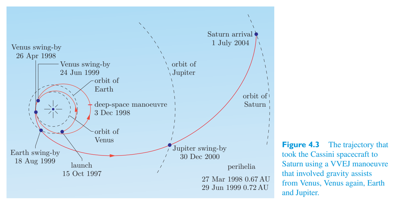
The Newtonian approach to gravitation has been so successful that many confuse Newton’s proposed explanation of gravitation with the phenomenon itself. The question ‘What is gravitation?’ deserves an answer that speaks of the general tendency of massive bodies to draw together, yet even today a common answer is that it is an attractive force described by an inverse square law. Newton’s brilliant and highly successful concept of a gravitational force has taken over gravitation in much the same way that the term ‘Hoover’ has replaced ‘vacuum cleaner’.牛顿的引力方法非常成功,以至于许多人将牛顿提出的引力解释与现象本身混为一谈。 “什么是引力?”这个问题需要一个关于大质量物体相互吸引的一般趋势的答案,但即使在今天,一个常见的答案仍然是它是一种由平方反比定律描述的吸引力。牛顿出色且非常成功的引力概念已经取代了万有引力,就像“胡佛”一词取代了“真空吸尘器”一样。
However, as Chapter 2 started to show, the development of Einsteinian relativity exposed problems deep in the heart of the Newtonian approach to gravitation. Under a change of inertial reference frame, a force described by an inverse square law does not transform in the way that a (three-) force should according to special relativity. Perhaps even more seriously, the Newtonian requirement that for every action there is an equal and opposite reaction implies that the gravitational forces linking two widely separated bodies should act instantly, irrespective of the distance between the two bodies. This is clearly at odds with the special relativistic requirement that such effects should not travel faster than the speed of light. Such arguments showed that Newtonian gravitation was not consistent with special relativity, and it soon became clear that no minor modification would make the two consistent.然而,正如第二章开始表明的那样,爱因斯坦相对论的发展暴露了牛顿引力理论的核心问题。在惯性参考系变化的情况下,由平方反比定律描述的力不会按照狭义相对论中的(三)力应有的方式变化。也许更严重的是,牛顿要求每一个作用都有一个相等且相反的反应,这意味着联络两个相距较远的物体的引力应该立即起作用,无论两个物体之间的距离如何。这显然与特殊相对论的要求相矛盾,即这种效应的传播速度不应超过光速。这些论证表明牛顿引力与狭义相对论不一致,而且很快人们就清楚,任何微小的修改都不能使两者一致。
The aim of this chapter is to introduce the core ideas of general relativity — Einstein’s relativistic theory of gravity. We start with the principles that guided Einstein in his search for the theory, then go on to examine the basic mathematical ingredients of the theory, and finally present the Einstein field equations that relate those ingredients and use them to provide a new explanation of gravitation that does not require the existence of any gravitational force.本章的目的是介绍广义相对论的核心思想——爱因斯坦的相对论引力理论。我们从引导爱因斯坦探索理论的原理开始,然后继续研究该理论的基本数学成分,最后提出将这些成分联系起来的爱因斯坦场方程,并用它们提供一种不需要任何引力存在的新的引力解释。
4.1 The founding principles of general relativity4.1 广义相对论的基本原理
Formulating a new theory in fundamental physics is not an entirely logical process. The search usually involves some general fundamental principles, consistency with known experimental facts, elegance and economy of ideas, and, inevitably, some guesswork. Of course, the ultimate test of any theory is provided by confronting its predictions with new experiments, and we shall come to this in Chapter 7; first we have to formulate the theory. Einstein was motivated in his search by three basic principles:在基础物理学中制定新理论并不是一个完全合乎逻辑的过程。搜索通常涉及一些一般的基本原则、与已知实验事实的一致性、思想的优雅和经济性,以及不可避免的一些猜测。当然,任何理论的最终检验都是通过新的实验来检验其预测,我们将在第七章中讨论这一点;首先我们必须阐述理论。爱因斯坦的研究受到三个基本原则的推动:
1. The principle of equivalence1. 等价原则
2. The principle of covariance2.协方差原理
3. The principle of consistency.3、一致性原则。
We shall discuss each of these in turn.我们将依次讨论这些内容。
4.1.1 The principle of equivalence4.1.1 等效原则
It was in 1907, just two years after the formulation of special relativity, that Einstein had the sudden insight that he later described as ‘the happiest thought of my life’. That thought was the realization that for an individual who was falling freely, accelerating downwards from a roof, say, or some other high place, it was almost as if gravity had been turned off. This idea, linking gravitation and acceleration, gave Einstein his start on extending relativity theory to include gravitation and showed him that a theory of general relative motion — one that included accelerations as well as uniform relative motions — could also be a theory of gravitation. This idea, that Einstein would later formalize as the principle of equivalence, also shed light on a troubling aspect of Newtonian mechanics.1907 年,即狭义相对论提出两年后,爱因斯坦突然有了顿悟,他后来将其描述为“我一生中最幸福的想法”。这个想法是这样的认识:对于一个自由落体的人来说,从屋顶或其他高处加速下降,几乎就像引力已经被关闭一样。这个将引力和加速度联系起来的想法使爱因斯坦开始将相对论扩展到包括引力,并向他表明广义相对运动理论(包括加速度和匀速相对运动)也可以是引力理论。爱因斯坦后来将这个想法形式化为等效原理,也揭示了牛顿力学的一个令人不安的方面。
The equality of gravitational and inertial mass引力质量和惯性质量相等
Newtonian mechanics involves two different concepts of mass:牛顿力学涉及两种不同的质量概念:
1. Inertial mass, m, which describes a particle’s resistance1. 惯性质量 m,描述粒子的阻力
to being accelerated by a force. The inertial mass of a particle is defined, according to Newton’s second law, by the ratio of the magnitude of the force on the m = | F |/| a |. particle to the magnitude of the acceleration it produces,被力加速。根据牛顿第二定律,粒子的惯性质量由作用在 m = | 上的力的大小之比来定义。 F|/|一个|。粒子产生的加速度的大小,
2. Gravitational mass, \(\mu\), which determines the force2. 引力质量,\(\mu\),它决定了力
that a given particle experiences due to, or exerts on, another particle as a result of gravity. The gravitational mass is defined through Newton’s law of gravitation for the force \(F^{12}\) on particle 1 of gravitational mass \(\mu\) 1 due to particle 2 of gravitational mass \((\mu)^2\). The magnitude of this force can be written as一个给定的粒子由于引力而受到另一个粒子的影响或施加在另一个粒子上。引力质量通过牛顿万有引力定律定义,即引力质量为 \(\mu\) 1 的粒子 1 由于引力质量为 \((\mu)^2\) 的粒子 2 所受的力 \(F^{12}\)。该力的大小可以写为
Now, as will be discussed later, it is a well-established experimental fact that the ratio \(\mu\)/m is the same for all bodies, to an accuracy of at least one part in \(10^{11}\). In Newtonian mechanics, this is simply an extraordinary coincidence with no explanation. However, for Einstein it was something that cried out for a fundamental explanation. Of course, once we accept that the ratio of gravitational to inertial mass is a constant, then we can (and do) choose to use units of measurement that make the two masses for any body equal, so that \(\mu\)/m = 1. This is why we can ignore the distinction between gravitational and inertial masses for almost all practical purposes.现在,正如稍后将讨论的,这是一个公认的实验事实,即比率 \(\mu\)/m 对于所有物体都是相同的,精度至少为 \(10^{11}\) 的一部分。在牛顿力学中,这只是一个非凡的巧合,无需解释。然而,对于爱因斯坦来说,这是迫切需要一个基本解释的事情。当然,一旦我们接受引力质量与惯性质量之比是一个常数,那么我们就可以(并且确实)选择使用使任何物体的两个质量相等的测量单位,使得 \(\mu\)/m = 1。这就是为什么我们可以在几乎所有实际目的中忽略引力质量和惯性质量之间的区别。
Freely falling frames are locally inertial frames自由落体框架是局部惯性系
In Newtonian physics, the equality of inertial and gravitational mass implies that the acceleration of any body due to a gravitational force is independent of the mass of the body.在牛顿物理学中,惯性质量和引力质量的相等意味着任何物体由于引力而产生的加速度与物体的质量无关。
- ● Prove the above statement.● 证明上述说法。
❍ The equality of inertial and gravitational mass implies that \(\mu\) i in Equation 4.1 may be replaced by m i, so❍ 惯性质量和引力质量相等意味着方程 4.1 中的 \(\mu\) i 可以用 m i 代替,因此
The acceleration a 1 of particle 1 due to this force is given by由于该力,粒子 1 的加速度 a 1 由下式给出
and hence因此
Clearly, the mass m 1 cancels, and consequently the acceleration of any body subject only to gravitational forces will be independent of the mass of the body.显然,质量 m 1 抵消,因此任何仅受引力作用的物体的加速度将与物体的质量无关。
This result leads us to consider a famous ‘thought experiment’ in which it is supposed that a frictionless (non-rotating) lift is falling freely down an airless lift shaft (see Figure 4.4). The acceleration of the lift or any object in the vicinity of the lift is independent of its mass. Consequently, for an observer inside the lift, an object released from rest (relative to the observer) would remain stationary; that is, according to the freely falling observer, the object would be free of any force and would continue in its state of rest. Moreover, if the observer were to exert a force on the object, it would move according to Newton’s laws of motion. In other words, from the point of view of the observer in the freely falling lift, a frame of reference fixed in the lift is an inertial frame of reference.这个结果让我们考虑一个著名的“思想实验”,其中假设一个无摩擦(非旋转)的电梯沿着无空气的电梯井自由下落(见图 4.4)。电梯或电梯附近任何物体的加速度与其质量无关。因此,对于电梯内的观察者来说,从静止状态释放的物体(相对于观察者)将保持静止;也就是说,根据自由落体观察者的说法,该物体将不受任何力的影响,并将继续处于静止状态。此外,如果观察者对物体施加力,物体就会根据牛顿运动定律移动。换句话说,从自由落体升降机中的观察者的角度来看,固定在升降机中的参考系是惯性参考系。
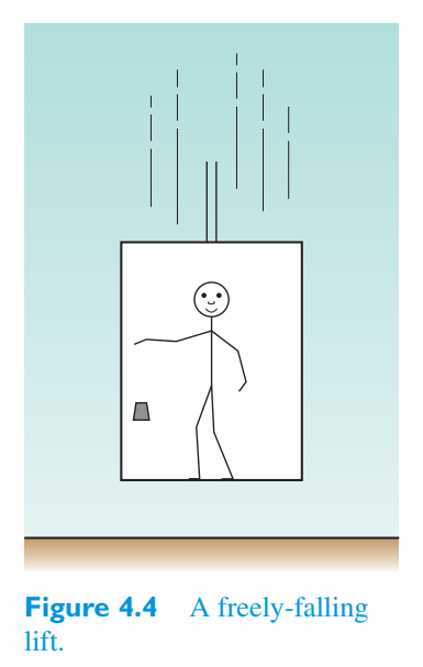
Such a frame is properly described as a locally inertial frame (as opposed to a globally inertial frame) because we need to restrict our measurements to sufficiently small regions of space and sufficiently small intervals of time if we are not to observe departures from inertial behaviour. This is because the gravitational field in which the lift and its contents are located is not uniform. Two objects released simultaneously from the same height on opposite sides of the lift will each fall towards the centre of the Earth, so instead of falling along parallel paths and maintaining a constant separation, as they would in a uniform gravitational field, they will in fact fall along converging paths and gradually approach each other. The horizontal forces responsible for this non-inertial behaviour are examples of the tidal forces that cause neighbouring particles in any non-uniform gravitational field to have different accelerations. Such effects are usually small but they can have observable consequences (such as the tides in the Earth’s oceans!), and even within a freely falling lift they would be observable if experiments were performed with sufficient precision or over a sufficiently long period of time. Nonetheless, the point remains that a freely falling frame in a gravitational field is a locally inertial frame where the laws of special relativity will hold true.这样的框架被正确地描述为局部惯性系(而不是全局惯性系),因为如果我们不观察惯性行为的偏离,我们需要将我们的测量限制在足够小的空间区域和足够小的时间间隔内。这是因为电梯及其内容物所在的引力场并不均匀。从升力两侧相同高度同时释放的两个物体将各自落向地球中心,因此它们不会像在均匀引力场中那样沿着平行路径下落并保持恒定的距离,而是实际上会沿着会聚路径下落并逐渐相互接近。导致这种非惯性行为的水平力是潮汐力的例子,潮汐力会导致任何非均匀引力场中的相邻粒子具有不同的加速度。这种效应通常很小,但可以产生可观察到的后果(例如地球海洋中的潮汐!),即使在自由落体的升力内,如果实验以足够的精度或在足够长的时间内进行,它们也是可以观察到的。尽管如此,问题仍然是,引力场中的自由落体框架是局部惯性系,狭义相对论定律在其中成立。
Exercise 4.1 Two objects are 2.00 m apart in a freely练习 4.1 两个物体在自由空间中相距 2.00 m
falling lift near to the surface of the Earth (which has a radius of \(6.38\times10^{6}\) m).接近地球表面的下降升力(半径为 \(6.38\times10^{6}\) 米)。
(a) Calculate the magnitude of their acceleration towards each other when their separation is horizontal.(a) 计算当它们水平分离时它们相对于彼此的加速度大小。
(b) Calculate the magnitude of their acceleration towards each other when their separation is vertical.(b) 计算当它们垂直分离时它们相对于彼此的加速度大小。
Of course, you might well ask what is meant by ‘sufficiently small’ for a frame to be locally inertial. The answer is that we assume that having decided on limits to the accuracy of a particular experiment, we can always choose a small enough region and a short enough time interval so that a freely falling frame will appear to be inertial to within this accuracy.当然,您可能会问框架具有局部惯性的“足够小”是什么意思。答案是,我们假设在决定了特定实验精度的限制后,我们总是可以选择足够小的区域和足够短的时间间隔,以便自由落体框架在这个精度内看起来是惯性的。
Another thought experiment involves a rocket in a region in which there is no gravitational field. If the rocket is accelerated with a uniform acceleration of magnitude g, no sufficiently localized experiment within the rocket can distinguish between the consequences of the acceleration and the gravitational field on the surface of the Earth. An object released from rest within the rocket would accelerate downwards, just as an object on Earth would do (see Figure 4.5).另一个思想实验涉及在没有引力场的区域中发射火箭。如果火箭以 g 级的均匀加速度加速,则火箭内没有足够的局部实验可以区分加速度和地球表面引力场的后果。火箭内从静止状态释放的物体会向下加速,就像地球上的物体一样(见图 4.5)。
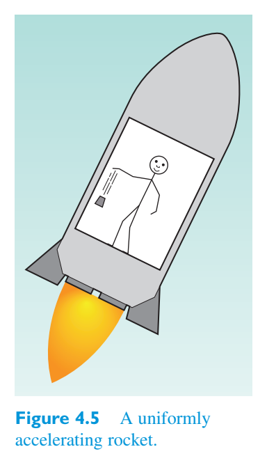
Principle of equivalence等效原理
In 1907, Einstein elevated to a formal principle the idea that locally one cannot distinguish between gravity and acceleration. What is now known as the weak equivalence principle can be stated as follows.1907 年,爱因斯坦将局部无法区分引力和加速度的想法提升为正式原则。现在所谓的弱等效原理可以表述如下。
Weak equivalence principle弱等价原理
Within a sufficiently localized region of spacetime adjacent to a concentration of mass, the motion of bodies subject to gravitational effects alone cannot be distinguished by any experiment from the motion of bodies within a region of appropriate uniform acceleration.在与质量集中相邻的足够局域化的时空区域内,任何实验都无法将仅受到引力作用的物体的运动与适当均匀加速度区域内的物体的运动区分开来。
The weak equivalence principle is a direct consequence of the fact that the acceleration of freely falling objects does not depend on their composition, and it is therefore sometimes referred to as the principle of universality of free fall. Note that this does not apply to very massive objects that would substantially change the gravitational field in their vicinity. Moreover, it only relates to gravitational forces, so experiments involving electromagnetic forces or nuclear interactions are specifically excluded.弱等效原理是自由落体物体的加速度不取决于其组成这一事实的直接结果,因此有时被称为自由落体普遍性原理。请注意,这不适用于会显着改变其附近引力场的非常大的物体。此外,它只与引力有关,因此涉及电磁力或核相互作用的实验被明确排除。
The restriction to gravitational forces does not apply to the strong equivalence principle.对引力的限制不适用于强等效原理。
Strong equivalence principle强等价原则
Within a sufficiently localized region of spacetime adjacent to a concentration of mass, the physical behaviour of bodies cannot be distinguished by any experiment from the physical behaviour of bodies within a region of appropriate uniform acceleration.在与质量集中相邻的足够局部的时空区域内,任何实验都无法将物体的物理行为与适当均匀加速度区域内的物体的物理行为区分开来。
This statement (which is often simply referred to as the equivalence principle) clearly goes beyond the universality of free fall, although that is included as a special case.这种说法(通常简称为等效原理)显然超出了自由落体的普遍性,尽管它被列为特例。
Both versions of the equivalence principle have been subject to many direct experimental tests. Galileo is often said to have demonstrated the universality of free fall by dropping different objects from the leaning tower of Pisa. It is unlikely that he actually performed such an experiment, but the experiments that he did perform — rolling bodies down inclined planes — should have made him aware of the outcome to expect. The first high-precision tests were carried out over many years with steadily improving sensitivity, eventually reaching better than one part in 10 8, by the Hungarian scientist Lora`nd Eo¨tvo¨s (pronounced ‘ert-vos’) in the late nineteenth and early twentieth centuries. These results were quoted by Einstein in his first complete formulation of general relativity. Currently, the most rigorous test of the weak equivalence principle is provided by the Eo¨t-Wash experiments, which provide agreement to better than one part in \(10^{12}\) (see Figure 4.6). Projected satellite experiments could provide even more stringent tests. For instance, the proposed Satellite Test of the Equivalence Principle (STEP), a space mission that is still in the design stage, could provide an accuracy of one part in \(10^{18}\).等效原理的两个版本都经过了许多直接的实验测试。人们常说伽利略通过从比萨斜塔上扔下不同的物体来证明自由落体的普遍性。他不太可能真的进行过这样的实验,但他所做的实验——让物体沿着斜面滚动——应该让他意识到预期的结果。十九世纪末二十世纪初,匈牙利科学家洛兰·埃奥特沃斯(Lora`nd Eo´tvo´s,发音为“ert-vos”)进行了多年的首次高精度测试,灵敏度稳步提高,最终达到了 10 8 分之一以上。爱因斯坦在他第一个完整的广义相对论中引用了这些结果。目前,Eo et-Wash 实验提供了对弱等效原理最严格的测试,该实验提供了比 \(10^{12}\) 中的一个部分更好的一致性(见图 4.6)。预计的卫星实验可以提供更严格的测试。例如,拟议的等效原理卫星测试(STEP)是一项仍处于设计阶段的太空任务,可以提供 \(10^{18}\) 中一个零件的精度。
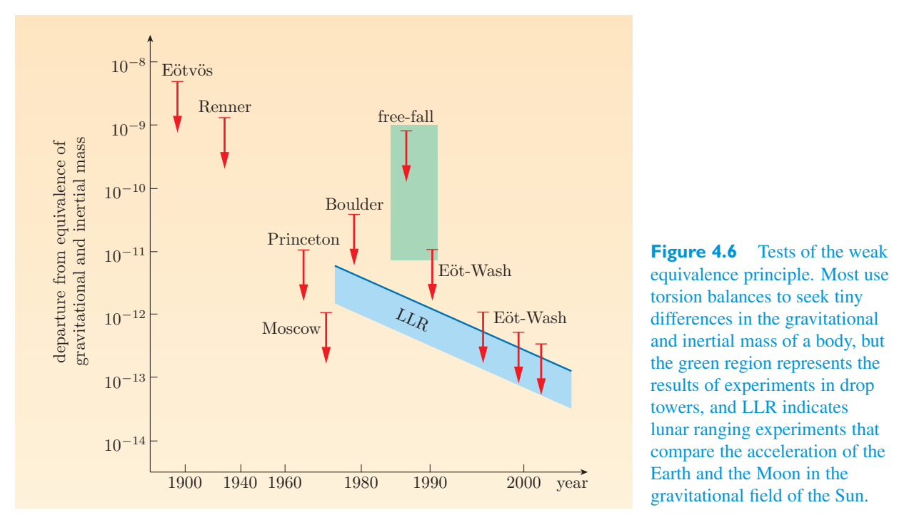
Experimental tests of the strong equivalence principle are much less clear-cut, but most theories that violate it predict that the locally measured value of the gravitational constant, G, may vary with time. Current constraints on the rate of change of G are approaching one part in \(10^{13}\) \(\mathrm{year^{-1}}\). Einstein’s theory of general relativity is thought to be the only theory of gravity that is consistent with the strong equivalence principle.强等效原理的实验测试不太明确,但大多数违反该原理的理论都预测,当地测量的引力常数 G 的值可能会随时间而变化。目前对G变化率的限制正在接近\(10^{13}\)年−1的一部分。爱因斯坦的广义相对论被认为是唯一符合强等效原理的引力理论。
Although the strong equivalence principle is certainly in need of additional tests, the weak equivalence principle alone was sufficient to lead Einstein to predict two new effects that eventually became part of general relativity. First, consider a horizontally travelling beam of light that enters and crosses the interior of a rocket that is accelerating vertically upwards — at right angles to the beam of light. From the point of view of the accelerated observer travelling with the rocket, the light ray follows a downward-curving path. The local equivalence of gravitation and acceleration therefore led Einstein to predict that one effect of gravitation would be the deflection of light rays towards concentrations of mass. The second effect was based on the fact that an observer in an upward-accelerating rocket would find that the frequency of light waves emitted from the floor of the rocket would be redshifted (i.e. their frequency would be decreased) as successive wave peaks took longer and longer to reach the ceiling. (These effects are illustrated in Figure 4.7.) This led Einstein to predict that light escaping from a concentration of mass should exhibit a redshift due to gravity. As you will see later, these two predicted effects, the gravitational deflection of light and the gravitational redshift of light, both became the subject of refined calculations in the full theory of general relativity and both eventually became important tests of the theory.尽管强等效原理肯定需要额外的测试,但仅弱等效原理就足以让爱因斯坦预测出两个新效应,最终成为广义相对论的一部分。首先,考虑一束水平行进的光束,该光束进入并穿过火箭内部,火箭垂直向上加速——与光束成直角。从随火箭行进的加速观察者的角度来看,光线遵循向下弯曲的路径。因此,引力和加速度的局部等效性使爱因斯坦预测引力的一种效应是使光线偏向质量集中。第二个效应基于这样一个事实:向上加速的火箭中的观察者会发现,随着连续的波峰到达天花板所需的时间越来越长,从火箭底部发射的光波的频率会发生红移(即它们的频率会降低)。(这些效应如图 4.7 所示。)这使得爱因斯坦预测,从质量集中逸出的光应该会因引力而表现出红移。正如你稍后将看到的,光的引力偏转和光的引力红移这两种预测效应都成为了整个广义相对论中精细计算的主题,并最终成为了该理论的重要检验。
The final form of general relativity was not clear to Einstein in 1907, but his realization that gravitation was in some sense locally equivalent to acceleration made the notion of a gravitational force suspect and the equivalence of gravitational and inertial mass almost a matter of course. The idea that a freely falling (accelerated) observer was equivalent to an inertial observer, at least locally, raised again the issue of coordinate transformations but made it clear that in general relativity the class of relevant coordinate transformations would have to be much broader than the Lorentz transformations of special relativity.1907 年,爱因斯坦还不清楚广义相对论的最终形式,但他意识到引力在某种意义上局部等同于加速度,这使得引力的概念受到怀疑,而引力和惯性质量的等同性几乎是理所当然的。自由落体(加速)观察者至少在局部相当于惯性观察者的想法再次提出了坐标变换的问题,但清楚地表明,在广义相对论中,相关坐标变换的类别必须比狭义相对论的洛伦兹变换广泛得多。
4.1.2 The principle of general covariance4.1.2 广义协方差原理
General covariance一般协方差
The principle of general covariance is an extension of the principle of relativity that was introduced in Chapter 1. According to the principle of relativity, the laws of physics should take the same form in all inertial frames. As you saw in Chapter 2, that implied that physical laws should be form-invariant under Lorentz transformations, and a way of ensuring that was to write the laws as properly balanced four-tensor relations. We saw how to do that for the laws of electromagnetism using scalar invariants (four-tensors of rank zero), contravariant and covariant four-vectors (four-tensors of rank 1), and some four-tensors of [F \(\mu\)\(\nu\)], the mixed field rank 2 — specifically, the contravariant field four-tensor four-tensor [F \(\mu\) \(\nu\)], and the covariant field four-tensor [F \(\mu\)\(\nu\)]. (Remember that when we enclose a tensor component in square brackets, it indicates that we are discussing the entire tensor, not just the individual component.) You will also recall that it was the principle of relativity that excluded Newtonian gravitation from being a viable relativistic theory of gravity; the Newtonian gravitational force cannot be described as part of a four-vector, because it does not transform in the right way.广义协变原理是第一章中介绍的相对论原理的延伸。根据相对论原理,物理定律在所有惯性系中应采取相同的形式。正如您在第二章中看到的,这意味着物理定律在洛伦兹变换下应该是形式不变的,确保这一点的一种方法是将定律写成适当平衡的四张量关系。我们看到了如何使用标量不变量(秩为 0 的四张量)、逆变和协变四向量(秩为 1 的四个张量)以及 [F \(\mu\)\(\nu\)] 的一些四张量、混合场秩 2 — 具体而言,逆变场四张量四张量 \([F^{\mu}]\) 来实现电磁定律。 \(\nu\)],以及协变场四张量 [F \(\mu\)\(\nu\)]。(请记住,当我们将张量分量括在方括号中时,这表明我们正在讨论整个张量,而不仅仅是单个分量。)您还会记得,正是相对论原理将牛顿引力排除在可行的相对论引力理论之外。牛顿引力不能被描述为四矢量量量的一部分,因为它没有以正确的方式变换。
The principle of general covariance extends the principle of relativity by requiring the physical equivalence of all frames, including non-inertial ones.广义协变原理通过要求所有框架(包括非惯性系)的物理等效性来扩展相对论原理。
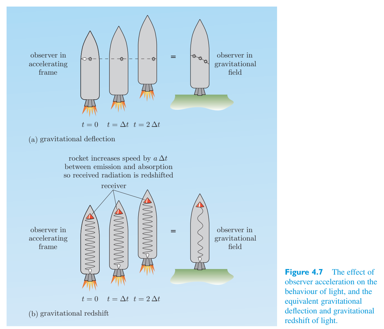
There is still debate about the significance of this principle and the extent to which Einstein was successful in implementing it in general relativity. However, what he did in practice was to require that physical laws should retain their form under a broad class of coordinate transformations, and he did this by requiring that the laws should be expressed in terms of mathematical objects called general tensors, or more often just tensors. Most of this section will be devoted to making clear what tensors are, how they differ from the more restricted four-tensors that you met in Chapter 2, and how they may be combined to form tensor equations that might describe generally covariant laws of physics, including gravitation.关于这一原理的重要性以及爱因斯坦在广义相对论中成功应用该原理的程度,仍然存在争议。然而,他在实践中所做的是要求物理定律应该在广泛的坐标变换下保持其形式,并且他通过要求物理定律应该用称为广义张量或更常见的张量的数学对象来表达来做到这一点。本节的大部分内容将致力于阐明张量是什么,它们与您在第 2 章中遇到的更受限制的四张量有何不同,以及如何将它们组合起来形成张量方程,这些方程可以描述一般的协变物理定律,包括万有引力。
Defining general tensors定义一般张量
The study of tensors can be approached in several ways, but for our purposes tensors are multi-component mathematical objects that can be recognized and classified according to the way their components behave under general coordinate transformations — that is, under coordinate transformations in which the new coordinates \(x'\) \(\mu\) are functions of the old coordinates x \(\nu\), as in \(x'\) \(\mu\) = \(x'\) \(\mu\) (x \(\nu\)) for \(\mu\), \(\nu\) = 0, 1, 2, 3. These functions are required to be sufficiently well-behaved that they can be differentiated, but they are still more general than the Lorentz transformations of special relativity, which were restricted to linear functions. In the case of the Lorentz transformations, the linearity ensured that derivatives such as ∂\(x'\) \(\mu\)/∂x \(\nu\) would be constants (such as c, V, γ or combinations of those parameters). In the case of a general coordinate transformation \(x'\) \(\mu\) = \(x'\) \(\mu\) (x \(\nu\)), the sixteen functions ∂\(x'\) \(\mu\)/∂x \(\nu\) (\(\mu\), \(\nu\) = 0, 1, 2, 3) and the sixteen functions ∂x \(\beta\)/∂\(x'\) \(\alpha\) (\(\alpha\), \(\beta\) = 0, 1, 2, 3) are free of such restrictions. Having explained what is meant by a general coordinate transformation, we can say that a tensor of contravariant rank m and covariant rank n has components \(T'\) \(\mu\) \(\alpha\) 1 \(\mu\) \(\alpha\) 2...\(\mu\)...\(\alpha\) m that transform according to张量的研究可以通过多种方式进行,但就我们的目的而言,张量是多分量数学对象,可以根据其分量在一般坐标变换下的行为方式进行识别和分类 - 也就是说,在坐标变换下,新坐标 \(x'\) \(\mu\) 是旧坐标 x \(\nu\) 的函数,如 \(x'\) \(\mu\) = \(x'\) \(\mu\) (x \(\nu\)) 对于 \(\mu\),\(\nu\) = 0, 1, 2, 3。这些函数需要表现得足够好才能被微分,但它们仍然比狭义相对论的洛伦兹变换更普遍,后者仅限于线性函数。在洛伦兹变换的情况下,线性确保诸如 ∂\(x'\) \(\mu\)/∂x \(\nu\) 之类的导数将是常数(例如 c、V、γ 或这些参数的组合)。在一般坐标变换 \(x'\) \(\mu\) = \(x'\) \(\mu\) (x \(\nu\)) 的情况下,十六个函数 ∂\(x'\) \(\mu\)/∂x \(\nu\) (\(\mu\), \(\nu\) = 0, 1, 2, 3) 和十六个函数∂x \(\beta\)/∂\(x'\) \(\alpha\) (\(\alpha\), \(\beta\) = 0, 1, 2, 3) 不受此类限制。解释了一般坐标变换的含义后,我们可以说逆变秩 m 和协变秩 n 的张量的分量 \(T'\) \(\mu\) \(\alpha\) 1 \(\mu\) \(\alpha\) 2...\(\mu\)...\(\alpha\) m 根据以下变换
Expressed in such general terms this looks very complicated, but the simple fact is that you have already met many of the most important tensor quantities that will be needed in this book. In particular, you are already familiar with the notion of a scalar invariant, S say, that remains unchanged under a general coordinate transformation. And you are also familiar with the infinitesimal displacement [d x \(\mu\)] = (d \(x^0\), d \(x^1\), \((dx)^2\), d \(x^{3}\)). This is actually a contravariant tensor of rank 1 with components that transform according to用这样的通用术语来表达,这看起来非常复杂,但简单的事实是,您已经满足了本书中需要的许多最重要的张量数量。特别是,您已经熟悉标量不变量的概念,例如 S,它在一般坐标变换下保持不变。您也熟悉无穷小位移 [d x \(\mu\)] = (d \(x^0\), d \(x^1\), \((dx)^2\), d \(x^{3}\))。这实际上是一个 1 阶逆变张量,其分量根据以下公式进行变换
You have also met the vastly important rank 2 metric tensor \(g_{\mu\nu}\). In its contravariant (dual) form its components transform according to您还遇到了极其重要的 2 阶度规张量 \(g_{\mu\nu}\)。在其逆变(对偶)形式中,其组件根据以下公式进行变换:
and in the covariant form they transform according to在协变形式中,它们根据
The metric tensor components satisfy the useful relationship度规张量分量满足有用关系
where δ \(\alpha\) \(\beta\) is a four-dimensional version of the Kronecker delta and is itself defined by其中 δ \(\alpha\) \(\beta\) 是克罗内克 delta 的四维版本,其本身定义为
1 if \(\alpha\) = \(\beta\), 0 if \(\alpha\) 3 = \(\beta\).如果 \(\alpha\) = \(\beta\),则为 1;如果 \(\alpha\),则为 0 3 = \(\beta\)。
You have even met the Riemann curvature tensor [R \(\alpha\) βγδ], a mixed tensor of contravariant rank 1 and covariant rank 3. In four-dimensional spacetime this tensor has 256 components, though due to symmetries, only 20 are independent. Each component transforms according to您甚至还遇到过黎曼曲率张量 [R \(\alpha\) βγδ],它是逆变 1 级和协变 3 级的混合张量。在四维时空中,该张量有 256 个分量,但由于对称性,只有 20 个分量是独立的。每个组件根据以下方式进行变换
A final point to note — or rather to recall, since it was mentioned in Chapter 3 — is that not all multi-component objects are tensors. It was pointed out earlier that the 64 connection coefficients Γ \(\alpha\) βγ of a four-dimensional spacetime do not satisfy the appropriate transformation law for a mixed rank 3 tensor, so they simply do not form a tensor.最后要注意的一点——或者更确切地说是回忆一下,因为它在第 3 章中提到过——是并非所有多分量对象都是张量。前面已经指出,四维时空的 64 个联络系数 Γ \(\alpha\) βγ 不满足混合阶 3 张量的适当变换定律,因此它们根本不构成张量。
Exercise 4.2 Suppose that in a two-dimensional Euclidean space with练习 4.2 假设在二维欧几里得空间中
coordinates x \(\mu\) (\(\mu\) = 1, 2) the coordinates \(x^1\) and \(x_{2}\) correspond to the polar coordinates r and \(\theta\). Also suppose that the coordinates \(x'\) \(\mu\) correspond to the usual Cartesian coordinates x, y.坐标x \(\mu\) (\(\mu\) = 1, 2) 坐标x 1 和x 2 对应于极坐标r 和\(\theta\)。还假设坐标 \(x'\) \(\mu\) 对应于通常的笛卡尔坐标 x, y。
(a) If A \(\mu\) is a general tensor component in r, \(\theta\) coordinates, and \(A'\) \(\mu\) is the corresponding tensor component in x, y coordinates, find the transformation that expresses \(A'\) \(\mu\) in terms of A \(\mu\) for each value of \(\mu\).(a) 如果 A \(\mu\) 是 r、\(\theta\) 坐标中的一般张量分量,并且 \(A'\) \(\mu\) 是 x、y 坐标中的相应张量分量,则对于 \(\mu\) 的每个值,找到用 A \(\mu\) 表示 \(A'\) \(\mu\) 的变换。
(b) Confirm that this transformation law is satisfied by the two-dimensional infinitesimal displacement vector that has components (d \(x^1\), \((dx)^2\)) = (d r, d \(\theta\)) and (d \(x'_{1}\), d \(x'_{2}\)) = (d x, d y).(b) 确认具有分量 (d \(x^1\), \((dx)^2\)) = (d r, d \(\theta\)) 和 (d \(x'_{1}\), d \(x'_{2}\)) = (d x, d y) 的二维无穷小位移矢量满足该变换定律。
Raising and lowering general tensor indices提高和降低一般张量指数
It is the metric tensor that relates contravariant and covariant tensor components via它是通过以下方式将逆变和协变张量分量关联起来的度规张量
and和
In other words, the contravariant metric tensor ‘raises’ indices and the covariant metric tensor ‘lowers’ them.换句话说,逆变度规张量“提高”指数,协变度规张量“降低”指数。
Exercise 4.3 Show that if we use the covariant metric tensor to ‘lower’ the练习 4.3 证明如果我们使用协变度规张量来“降低”
index on A \(\mu\) and then we use the contravariant metric tensor to ‘raise’ the index again, we get back to A \(\mu\).A \(\mu\) 上的索引,然后我们使用逆变度规张量再次“提高”索引,我们回到 A \(\mu\)。
- ● If we have a mixed tensor with some indices up and some down, it is usually如果我们有一个混合张量,其中一些索引向上,一些索引向下,通常是
important to leave spaces so that, for example, we write R \(\alpha\) βγδ rather than R βγδ \(\alpha\). Explain why.留出空格很重要,例如,我们写 R \(\alpha\) βγδ 而不是 R βγδ \(\alpha\)。解释一下为什么。
❍ Suppose that we start with R αβγδ, then use the contravariant metric tensor to raise the \(\alpha\) index without paying attention to the order of the indices. We will obtain the result R βγδ \(\alpha\). The problem is that the individual indices are just placeholders and have no special significance. This means that if we subsequently use the covariant metric tensor to lower the \(\alpha\) index, it is impossible to tell if the lowered index should be put in the first or second ‘slot’, i.e. whether the result should be R αβγδ or R βαγδ. Unless the tensor happens to be symmetric with respect to interchange of the first two indices, the two possible results will be different. It is therefore usually important to preserve the order of the indices despite any raising or lowering that may be \(\alpha\) βγδ rather than R βγδ \(\alpha\). performed. That’s why we should generally write R❍ 假设我们从 R αβγδ 开始,然后使用逆变度规张量来提高 \(\alpha\) 索引,而不注意索引的顺序。我们将得到结果 R βγδ \(\alpha\)。问题是各个指数只是占位符,没有特殊意义。这意味着,如果我们随后使用协变度规张量来降低 \(\alpha\) 指数,则无法判断降低后的指数应该放在第一个还是第二个“槽”中,即结果应该是 R αβγδ 还是 R βαγδ。除非张量恰好关于前两个索引的互换对称,否则两个可能的结果将会不同。因此,尽管可能是 \(\alpha\) βγδ 而不是 R βγδ \(\alpha\),但保持索引的顺序通常很重要。执行。这就是为什么我们一般应该写 R
The rules of tensor algebra张量代数规则
Einstein’s aim was to use tensors to write down a theory of gravity in a generally covariant form — in other words, following the rules of general tensor algebra for multiplying tensors by scalars, adding and subtracting tensors, multiplying tensors together and reducing the rank of a tensor through contraction. These rules are similar to those that we have already used to manipulate four-tensors in special relativity, but to make them completely clear, we now list them in their general forms.爱因斯坦的目标是使用张量以一般协变的形式写下引力理论——换句话说,遵循一般张量代数的规则,将张量乘以标量、加减张量、将张量相乘以及通过收缩降低张量的阶。这些规则与我们已经用来操纵狭义相对论中的四张量的规则类似,但为了使它们完全清晰,我们现在以一般形式列出它们。
1. Scaling A tensor [T \(\mu\) 1 \(\alpha\) \((\mu)^2\) \(\alpha\)...\(\mu\)...\(\alpha\) m] of contravariant1. 逆变张量 [T \(\mu\) 1 \(\alpha\) \((\mu)^2\) \(\alpha\)...\(\mu\)...\(\alpha\) m] 的缩放
rank m and covariant rank n may be multiplied by a scalar S to produce a new tensor [U \(\mu\) 1 \(\alpha\) \((\mu)^2\) \(\alpha\)...\(\mu\)...\(\alpha\) m] of the same rank. Each component of the new tensor is obtained by multiplying the corresponding component of the original tensor by the same scalar S. So, for example, for all values of \(\mu\) and \(\alpha\),阶 m 和协变阶 n 可以乘以标量 S 以产生相同阶的新张量 [U \(\mu\) 1 \(\alpha\) \((\mu)^2\) \(\alpha\)...\(\mu\)...\(\alpha\) m]。新张量的每个分量都是通过将原始张量的相应分量乘以相同的标量 S 获得的。因此,例如,对于 \(\mu\) 和 \(\alpha\) 的所有值,
2. Addition and subtraction Tensors may be added2. 加法和减法张量可以相加
or subtracted to form new tensors, but those being added or subtracted must be of the same type, i.e. with the same contravariant rank and the same covariant rank. Again the addition or subtraction is carried out component by component. So, for example, for all values of \(\mu\) and \(\alpha\),或相减以形成新的张量,但相加或相减的张量必须是同一类型,即具有相同的逆变秩和相同的协变秩。同样,加法或减法是逐个分量地进行的。因此,例如,对于 \(\mu\) 和 \(\alpha\) 的所有值,
3. Multiplication Tensors may be multiplied together3. 乘法张量可以相乘
by forming products of \([X^{\mu}]\), [Y \(\alpha\)] and [Z \(\beta\)], their components. So, for example, given three tensors we can form a new tensor [A \(\mu\) αβ] with components通过形成产品\([X^{\mu}]\)、\([Y^{\alpha}]\)和\([Z^{\beta}]\)及其组件。因此,例如,给定三个张量,我们可以形成一个新的张量 [A \(\mu\) αβ],其分量
The rank of the new tensor is then the sum of the ranks of the tensors being multiplied together (e.g. A \(\mu\) αβ has rank 3). The tensors being multiplied together may even be the same, as in新张量的秩就是张量的秩相乘的总和(例如 \(\mu\) αβ 的秩为 3)。相乘的张量甚至可能是相同的,如
4. Contraction In the case of a single tensor with4. 收缩在单个张量的情况下
contravariant rank m and covariant rank n, or in the case of a product of tensors with combined contravariant rank m and covariant rank n, it is possible to form another tensor, of contravariant rank \(\mathrm{m^{-1}}\) and covariant rank n − 1, by summing over one raised index and one lowered index. So, for example,逆变等级 m 和协变等级 n,或者在张量与逆变等级 m 和协变等级 n 组合的乘积的情况下,可以通过对一个升高的索引和一个降低的索引求和来形成逆变等级 \(\mathrm{m^{-1}}\) 和协变等级 n − 1 的另一个张量。所以,举例来说,
These rules imply that tensors can appear in expressions only in certain well-defined ways. In order to illustrate this, consider the following (fairly arbitrary) equation involving tensors:这些规则意味着张量只能以某些明确定义的方式出现在表达式中。为了说明这一点,请考虑以下涉及张量的(相当任意的)方程:
The right-hand side of Equation 4.8 consists of the sum of three ‘terms’, which we can use to emphasize some important general properties of tensor equations.方程 4.8 的右侧由三个“项”之和组成,我们可以用它来强调张量方程的一些重要的一般性质。
- • The only indices that are not ‘summed over’ are \(\mu\) and \(\nu\). These are the free唯一未“汇总”的指数是 \(\mu\) 和 \(\nu\)。这些都是免费的
indices. They exhibit the following properties:指数。它们具有以下特性:
(a) The \(\mu\) and \(\nu\) indices are consistently ‘up’ (contravariant) or ‘down’ (covariant).(a) \(\mu\) 和 \(\nu\) 指数始终“上升”(逆变)或“下降”(协变)。
(b) The \(\mu\) and \(\nu\) indices appear once and only once in every term on each side of the equation.(b) \(\mu\) 和 \(\nu\) 指数在方程每边的每一项中出现且仅出现一次。
(c) The letters \(\mu\) and \(\nu\) have no special significance. We can replace either (or both) of them with a different (Greek) letter provided that we carry out the replacement in every term (on both sides of the equation) and the new letter does not clash with one that is already in use. For example, we could replace \(\mu\) with \(\lambda\), but replacing \(\mu\) with \(\alpha\) would cause confusion.(c) 字母 \(\mu\) 和 \(\nu\) 没有特殊意义。我们可以用不同的(希腊)字母替换其中一个(或两个),前提是我们在每一项(等式两边)中进行替换,并且新字母不会与已使用的字母发生冲突。例如,我们可以将 \(\mu\) 替换为 \(\lambda\),但将 \(\mu\) 替换为 \(\alpha\) 会导致混乱。
- • Some indices (\(\alpha\) and \(\beta\) in this example) appear precisely twice in a term. These某些索引(本例中为 \(\alpha\) 和 \(\beta\))在一个术语中恰好出现两次。这些
are the dummy indices.是虚拟指数。
(a) Such indices are always summed over.(a) 这些指数总是相加的。
(b) One appearance is always ‘up’ and the other is ‘down’.(b) 一种外观总是“向上”,另一种外观总是“向下”。
(c) The letter used has no special significance and can always be replaced with another (Greek) letter provided that we replace both occurrences within any one term and the new letter doesn’t clash with one that is already in use. For example, \(\alpha\) in the third term on the right-hand side could be replaced with γ, but not with \(\beta\).(c) 所使用的字母没有特殊意义,并且始终可以用另一个(希腊)字母替换,前提是我们替换任何一个术语中出现的两个字母,并且新字母不会与已使用的字母发生冲突。例如,右侧第三项中的α可以用γ代替,但不能用β代替。
As you can see, the indices within a covariant equation form very distinct patterns that you will soon become adept at spotting. Expressions such as Equation 4.8 are said to be generally covariant or, more simply, in covariant form. This means that the equation will take the same form in any coordinate system; it does not, of course, mean that the numerical values of the components are necessarily the same. It is worth noticing how the word ‘covariant’ is a bit over-used. A rank 1 ‘covariant tensor’ is one with components that transform according to正如您所看到的,协变方程中的索引形成了非常独特的模式,您很快就会熟练地发现这些模式。诸如方程 4.8 之类的表达式通常被认为是协变的,或者更简单地说,是协变形式的。这意味着该方程在任何坐标系中都将采用相同的形式;当然,这并不意味着各分量的数值必须相同。值得注意的是,“协变”这个词有点被过度使用了。 1 阶“协变张量”是一个其分量根据以下公式进行变换的张量:
and is denoted by having the indices ‘down’. A ‘covariant equation’ is an equation that takes the same form in different coordinate systems, and may or may not involve covariant tensors. Indeed, a covariant equation may involve contravariant tensors.并通过指数“下降”来表示。 “协变方程”是在不同坐标系中采用相同形式的方程,并且可能涉及也可能不涉及协变张量。事实上,协变方程可能涉及逆变张量。
- ● What is the analogous equation to Equation 4.9 that describes how the与方程 4.9 类似的方程描述了如何
components of a rank 1 contravariant tensor transform?1 阶逆变张量变换的组成部分?
❍ From Equation 2.110 or from the rank 1 example that follows it in Equation 4.2, the required transformation rule is❍ 根据公式 2.110 或公式 4.2 中的秩 1 示例,所需的变换规则为
Exercise 4.4 Explain why each of the following is not练习 4.4 解释为什么下列各项不成立
a generally covariant tensor equation. Y \(\mu\)\(\nu\) Z \(\nu\) (c) A = (a) A \(\mu\) = B + K (b) X \(\mu\) =一般协变张量方程。 Y \(\mu\)\(\nu\) Z \(\nu\) (c) A = (a) A \(\mu\) = B + K (b) X \(\mu\) =
The rules of covariant differentiation协变微分的规则
When we wrote down the laws of Lorentz-covariant electromagnetism in Chapter 2, in addition to scaling, adding, multiplying and contracting four-tensors, we also formed four-tensors by taking partial derivatives of existing tensors. Being able to represent derivatives of four-tensors was important because the basic laws of electromagnetism (the Maxwell equations and the equation of continuity) were differential equations. We should expect the generally covariant theory of gravitation to involve differential equations, so we need to know how to differentiate a general tensor in a covariant way. This turns out to be more complicated in general relativity than it was in special relativity because simple partial derivatives of tensors are not generally covariant.当我们在第二章写下洛伦兹协变电磁学定律时,除了对四张量进行缩放、加法、乘法和收缩之外,我们还通过对现有张量求偏导数来形成四张量。能够表示四张量的导数非常重要,因为电磁学的基本定律(麦克斯韦方程和连续性方程)是微分方程。我们应该期望广义协变引力理论涉及微分方程,因此我们需要知道如何以协变的方式微分广义张量。事实证明,广义相对论中的情况比狭义相对论中的情况更为复杂,因为张量的简单偏导数通常不是协变的。
Defining the derivative of a function involves evaluating the function at some point, x say, and at a nearby point, x + δx say, and then taking the difference. In a flat space this does not present any particular problem. Nor is it particularly complicated in a curved space as long as we are only considering functions. vector [v \(\alpha\)] (i.e. a rank 1 However, we know from Chapter 3 that transporting a tensor) requires some care since the parallel transport of a vector generally involves the connection coefficients定义函数的导数涉及在某个点(例如 x)和附近的点(例如 x + δx)评估函数,然后求差。在平坦的空间中,这不会出现任何特殊问题。只要我们只考虑函数,在弯曲空间中也不是特别复杂。向量 \([v^{\alpha}]\) (即a 等级 1 然而,我们从第 3 章知道,传输张量需要小心,因为向量的并行传输通常涉及联络系数
For a vector with components v \(\alpha\), the expression对于具有分量 v \(\alpha\) 的向量,表达式
simply does not transform in the right way under general coordinate transformations to be a component of a rank 2 tensor. Nor does the expression在一般坐标变换下,根本无法以正确的方式变换为 2 阶张量的组成部分。表达式也不
However, sums of the form然而,形式的总和
arise when considering the limit of a difference in a vector and its parallel transported version, and this quantity does transform as a component of a rank 2 tensor. Expressions of this kind occur so frequently in general relativity that it is useful to give them a name and a symbol. Consequently, we write当考虑向量及其并行传输版本的差异极限时,就会出现这种情况,并且该量确实会变换为 2 阶张量的组成部分。这种表达式在广义相对论中出现得非常频繁,因此给它们命名和符号是很有用的。因此,我们写
and say that ∇ \(\beta\) v \(\alpha\) represents the covariant derivative of v \(\alpha\). In effect, the behaviour of ∂v \(\alpha\)/∂x \(\beta\) is cancelled by the non-tensorial behaviour non-tensorial, of \(\lambda\) Γ \(\alpha\) \(\lambda\)\(\beta\) v \(\lambda\). At this stage, you should regard ∇ \(\beta\) v \(\alpha\) as no more than a shorthand for the right-hand side of Equation 4.11. Of course, we don’t just want to differentiate rank 1 contravariant tensors. We also need to know how to covariantly differentiate rank 1 covariant tensors and tensors of higher rank, so that the result is a tensor in each case. It can be shown that Equation 4.11 implies that the covariant derivative of a covariant tensor v \(\alpha\) can be expressed as并称 ∇ \(\beta\) v \(\alpha\) 表示 v \(\alpha\) 的协变导数。实际上,∂v \(\alpha\)/∂x \(\beta\) 的行为被 \(\lambda\) Γ \(\alpha\) \(\lambda\)\(\beta\) v \(\lambda\) 的非张量行为抵消。在此阶段,您应该将 ∇ \(\beta\) v \(\alpha\) 视为公式 4.11 右侧的简写。当然,我们不仅仅想区分 1 阶逆变张量。我们还需要知道如何协变区分 1 阶协变张量和更高阶的张量,以便在每种情况下结果都是一个张量。可以看出,方程 4.11 意味着协变张量 v \(\alpha\) 的协变导数可以表示为
Note that in this case the final term is subtracted from the partial derivative, whereas in the case of a contravariant vector it was added. The covariant derivatives of higher-rank tensors are direct generalizations of Equations 4.11 and 4.12, as appropriate. For instance,请注意,在这种情况下,从偏导数中减去最后一项,而在逆变向量的情况下,最后一项被添加。高阶张量的协变导数是方程 4.11 和 4.12 的直接推广(视情况而定)。例如,
- ● Write down the expression for ∇ \(\lambda\) T \(\mu\) \(\nu\) in terms of the connection coefficients.用联络系数写出 ∇ \(\lambda\) T \(\mu\) \(\nu\) 的表达式。
❍ From Equations 4.11 and 4.12, we have❍ 根据方程 4.11 和 4.12,我们有
This is a good point at which to restate the principle of general covariance and summarize its significance in the formulation of general relativity.这是重申广义协变原理并总结其在广义相对论表述中的重要性的好时机。
General covariance, tensors and covariant differentiation一般协方差、张量和协变微分
According to the principle of general covariance, the laws of physics should take the same form in all frames of reference. In practice this means that they should be expressed as balanced tensor relationships that are covariant under general coordinate transformations.根据广义协变原理,物理定律在所有参考系中应采取相同的形式。实际上,这意味着它们应该表示为在一般坐标变换下协变的平衡张量关系。
Legitimate algebraic operations involving tensors include scaling, addition and subtraction (provided that the types are identical), multiplication and contraction. The partial differentiation of a tensor does not generally produce another tensor, but the process of covariant differentiation does. This may be applied to a tensor of any rank and is exemplified by涉及张量的合法代数运算包括缩放、加法和减法(前提是类型相同)、乘法和收缩。张量的偏微分通常不会产生另一个张量,但协变微分的过程会产生。这可以应用于任何阶的张量,例如
Exercise 4.5 What is the covariant derivative of the invariant scalar function练习 4.5 什么是不变标量函数的协变导数
S (ct, x, y, z)? (Hint: This is a tensor of rank 0.)S(ct、x、y、z)? (提示:这是一个 0 阶张量。)
4.1.3 The principle of consistency4.1.3 一致性原则
The principle of consistency asserts that a new theory that aims to replace or supersede earlier theories should account for the successful predictions of those earlier theories. In the particular case of general relativity, we should expect consistency with the successes of Einstein’s own special relativity and Newtonian gravitation. The former requirement is guaranteed by using a spacetime that is locally equivalent to Minkowski spacetime; the latter provides a useful constraint on the kinds of tensor equations that can be used in the formulation of general relativity.一致性原则主张,旨在取代或取代早期理论的新理论应该解释那些早期理论的成功预测。在广义相对论的特殊情况下,我们应该期望与爱因斯坦自己的狭义相对论和牛顿引力的成功保持一致。前一个要求是通过使用局部等价于闵可夫斯基时空的时空来保证的;后者对可用于广义相对论公式的张量方程类型提供了有用的约束。
For the purposes of establishing consistency with Newtonian predictions, it is helpful to first see how Newton’s theory of gravity, as expressed by the inverse square law, can be reformulated as a field theory, based on the idea of a gravitational field that obeys differential equations similar to those satisfied by the electric and magnetic fields of electromagnetism.为了与牛顿预测保持一致,首先了解牛顿的引力理论(以平方反比定律表示)如何可以重新表述为场论,基于引力场的思想,该引力场服从与电磁场的电场和磁场所满足的微分方程类似的微分方程,这是有帮助的。
field g (r) to be a To this end, we first define the Newtonian gravitational function of position r = (x, y, z) that specifies the Newtonian gravitational force per unit mass that would act on a test particle at the point r. This means that the be m g (r). It follows gravitational force on a particle of mass m at r would from Newton’s law of gravitation (Equation 4.1) that in the case of a uniform coordinates (r = 0), the spherical body of total mass M centred on the origin of gravitational field is given by场 g (r) 为 a 为此,我们首先定义位置 r = (x, y, z) 的牛顿引力函数,该函数指定在 r 点作用于测试粒子的每单位质量的牛顿引力。这意味着是 m g (r)。根据牛顿万有引力定律(方程 4.1),在统一坐标(r = 0)的情况下,以引力场原点为中心的总质量为 M 的球体由下式给出:
where e r is a unit vector in the radial direction, pointing away from the origin. The minus sign in Equation 4.14 means that g (r) is directed towards the origin at every point, as shown in Figure 4.8.其中 e r 是径向方向的单位向量,指向远离原点的方向。公式 4.14 中的负号表示 g(r) 在每一点都指向原点,如图 4.8 所示。
If we suppose that the sphere of mass M is enclosed by a larger sphere of radius R also centred on the origin, we can define the flux of the gravitational field leaving the larger sphere by a surface integral:如果我们假设质量为 M 的球体被一个同样以原点为中心、半径为 R 的较大球体包围,我们可以通过表面积分定义离开较大球体的引力场通量:
outward gravitational flux = g · n E d S,向外引力通量 = g·n E d S,
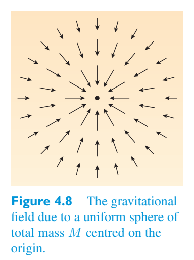
where n E is an outward-pointing unit vector normal to the spherical surface at every point. From the spherical symmetry of the situation, it is easy to see that in this case the surface integral will be given by the surface area of the sphere (4 πR 2) multiplied by the constant field strength on the surface of the sphere (GM/\(R^2\)), multiplied by − 1 because in this case the field points inwards, so e · n E = − 1. Thus其中 n E 是每个点垂直于球面的指向外的单位向量。从球对称的情况,很容易看出,在这种情况下,表面积分将由球体表面积 (4 πR 2) 乘以球体表面上的恒定场强 (GM/\(R^2\)) 得出,再乘以 − 1,因为在这种情况下场指向内,因此 e · n E = − 1。
Now, according to the divergence theorem of vector calculus, this kind of surface integral of the field can be rewritten as a volume integral of a quantity known as the divergence of the field, ∇ · g, throughout the volume现在,根据矢量微积分的散度定理,这种场的表面积分可以重写为整个体积中称为场散度 ∇·g 的量的体积积分
! where, in terms B of Cartesian components, the vector operator ∇ represents!其中,用笛卡尔分量 B 表示,向量算子 ∇ 表示
∂, ∂, ∂, so the divergence is defined by∂, ∂, ∂,因此散度定义为
If we now write the mass of the sphere as an integral over its density \(\rho\), we have如果我们现在将球体的质量写成其密度 \(\rho\) 的积分,我们有
Though not a proof, this last relation at least makes plausible a general relationship that can be proved by more rigorous methods, namely the differential relationship虽然不是证明,但最后一个关系至少使可以通过更严格的方法证明的一般关系变得合理,即微分关系
This is actually one of the fundamental equations of Newtonian gravitation, relating derivatives of the gravitational field to the mass density that is the source of the field. It is not restricted to spherical bodies, nor even to cases where the density is uniform. Nor is it quite the end of our argument.这实际上是牛顿引力的基本方程之一,将引力场的导数与作为场源的质量密度联系起来。它不限于球体,甚至也不限于密度均匀的情况。我们的争论还没有结束。
The gravitational force is conservative. That means that the work done against the gravitational force in moving a body from one point to another is independent of the path followed. That’s why it is possible to associate the gravitational force with a gravitational potential energy. The gravitational field g (r) can be similarly related to a gravitational potential field Φ(r) that describes the gravitational potential energy per unit mass located at r. The precise relationship is usually written in terms of a gradient as万有引力是保守的。这意味着将物体从一点移动到另一点时抵抗引力所做的功与所遵循的路径无关。这就是为什么可以将引力与引力势能联系起来。引力场 g (r) 可以类似地与描述位于 r 处每单位质量的引力势能的引力势场 Φ(r) 相关。精确的关系通常用梯度表示为
Substituting Equation 4.19 into Equation 4.18 leads to将公式 4.19 代入公式 4.18 得出
The combination ∇ · ∇ occurs so frequently in some areas of mathematics and physics that it is given a name, the Laplacian operator, and denoted by the symbol ∇ 2. Following this convention we can say that组合 ∇ · ∇ 在数学和物理的某些领域中出现得如此频繁,以至于它被命名为拉普拉斯算子,并用符号 ∇ 2 表示。按照这个约定,我们可以说:
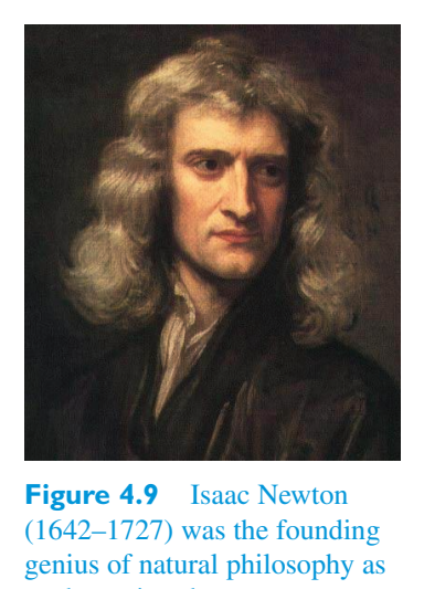
Written out in full, in terms of Cartesian coordinates, this equation says that用笛卡尔坐标完整写出,该方程表示
Equation 4.21 is called Poisson’s equation. It provides the essential summary of Newtonian gravitation in terms of a differential equation that we have been seeking. It is entirely equivalent to Newton’s inverse square law but has the advantage that it is a differential equation for a scalar quantity that may be straightforward to solve. The gravitational field (which is a vector) can then be obtained via Equation 4.19, which involves differentiating the scalar field Φ(r). Notice that both the gravitational potential Φ and the mass density \(\rho\) are functions of the same position variable r.方程 4.21 称为泊松方程。它以我们一直在寻找的微分方程形式提供了牛顿引力的基本总结。它完全等价于牛顿平方反比定律,但优点是它是一个标量的微分方程,可以直接求解。然后可以通过方程 4.19 获得引力场(矢量),其中涉及标量场 Φ(r) 的微分。请注意,引力势 Φ 和质量密度 \(\rho\) 都是同一位置变量 r 的函数。
Poisson’s equation and gravitation泊松方程和引力
The essence of Newtonian gravitation as a field theory is expressed in the Poisson equation牛顿引力场论的本质用泊松方程来表达
which relates a combination of second derivatives of the Newtonian gravitational potential Φ to the mass density \(\rho\) that is the source of the Newtonian gravitational field. The Newtonian gravitational field g is related to Φ by它将牛顿引力势 Φ 的二阶导数的组合与质量密度 \(\rho\) 联系起来,质量密度是牛顿引力场的来源。牛顿引力场 g 与 Φ 的关系为
It will be shown later that general relativity predicts that an equation of this type provides an approximate description of gravitation under appropriate circumstances (usually referred to as the Newtonian limit). It is in this sense that general relativity is consistent with the successful predictions of Newtonian gravitation, even though it makes no use of gravitational forces. General relativity is also consistent with special relativity in the sense that the results of special relativity hold true locally in general relativity.稍后将表明,广义相对论预测此类方程在适当的情况下(通常称为牛顿极限)提供了对引力的近似描述。正是在这个意义上,广义相对论与牛顿引力的成功预言是一致的,尽管它没有使用引力。广义相对论也与狭义相对论一致,因为狭义相对论的结果在广义相对论中局部成立。
4.2 The basic ingredients of general relativity4.2 广义相对论的基本要素
The principles outlined in the previous section led Einstein to formulate general relativity using covariant tensor equations. But what tensor quantities should be involved in those equations? It was obvious that a theory of gravity should involve the distribution of matter, and it was part of Einstein’s genius to realize that if gravity was somehow built into the geometric structure of spacetime, then it would act equally on all forms of matter and the universality of free fall would cease to be an unexplained accident. All forms of matter are subject to the same spacetime geometry, even though they may not be subject to identical forces. Such thoughts eventually led Einstein to consider two particular tensors as basic ingredients of general relativity — one describing the properties of matter, the other concerned with aspects of spacetime geometry. This section introduces those two tensor quantities and relates them to other tensors with which you are already familiar.上一节概述的原理引导爱因斯坦使用协变张量方程来制定广义相对论。但是这些方程中应该涉及哪些张量呢?显然,引力理论应该涉及物质的分布,爱因斯坦的天才之一是意识到,如果引力以某种方式构建到时空的几何结构中,那么它就会平等地作用于所有形式的物质,自由落体的普遍性将不再是一个无法解释的偶然事件。所有形式的物质都受到相同的时空几何形状的影响,尽管它们可能不会受到相同的力的影响。这些想法最终导致爱因斯坦将两个特定的张量视为广义相对论的基本成分——一个描述物质的属性,另一个涉及时空几何的各个方面。本节介绍这两个张量,并将它们与您已经熟悉的其他张量联系起来。
4.2.1 The energy–momentum tensor4.2.1 能量-动量张量
In Newton’s theory of gravity, mass, or more generally mass density, is a conserved quantity that is the ‘source’ of gravitation. (See, for instance Equation 4.21.) In special relativity, the mass m of a particle is no longer conserved, but it is related to the energy and momentum magnitude of the particle by在牛顿的引力理论中,质量,或更普遍的质量密度,是一个守恒量,是引力的“来源”。 (例如,参见方程 4.21。)在狭义相对论中,粒子的质量 m 不再守恒,但它与粒子的能量和动量大小相关:
and there are conservation laws that relate to energy (including mass–energy) and to momentum. Hence we should expect that in a relativistic theory, the source of gravitation cannot be mass alone but must also involve energy and momentum. Since these sources of gravitation must somehow appear in a tensor, you will not be surprised to learn that one of the basic ingredients of general relativity is known as the energy–momentum tensor. The only issues are: what is it, what is its rank, what are its symmetries, and how is it defined?并且存在与能量(包括质能)和动量相关的守恒定律。因此,我们应该预料到,在相对论理论中,引力的来源不能只是质量,还必须涉及能量和动量。由于这些引力源必须以某种方式出现在张量中,因此当您得知广义相对论的基本成分之一被称为能量-动量张量时,您不会感到惊讶。唯一的问题是:它是什么,它的等级是什么,它的对称性是什么,以及它是如何定义的?
The energy–momentum tensor describes the distribution and flow of energy and momentum in a region of spacetime. It is a rank 2 tensor, so at an event (i.e. any ‘point’ in spacetime) it is specified by sixteen components, usually denoted \(T_{\mu\nu}\) (\(\mu\), \(\nu\) = 0, 1, 2, 3). It is a symmetric tensor, so \(T_{\mu\nu}\) = T \(\nu\)\(\mu\), and that means that only ten of its components are independent (the four components T \(\mu\)\(\mu\) and six of the twelve components \(T_{\mu\nu}\) where \(\mu\) 3 = \(\nu\)). Each component can be measured in units of energy density (\(\mathrm{J\,m^{-3}}\)), though it is sometimes appropriate to use other equivalent units. Each component is a function of the spacetime coordinates, with the following general significance in the neighbourhood of each event in spacetime:能量-动量张量描述了时空区域中能量和动量的分布和流动。它是一个 2 阶张量,因此在一个事件(即时空中的任何“点”)上,它由 16 个分量指定,通常表示为 \(T_{\mu\nu}\)(\(\mu\)、\(\nu\) = 0, 1, 2, 3)。它是一个对称张量,因此 \(T_{\mu\nu}\) = T \(\nu\)\(\mu\),这意味着它只有 10 个分量是独立的(四个分量 T \(\mu\)\(\mu\) 和 12 个分量中的 6 个 \(T_{\mu\nu}\),其中 \(\mu\) 3 = \(\nu\))。每个成分都可以用能量密度单位 (\(\mathrm{J\,m^{-3}}\)) 来测量,尽管有时使用其他等效单位也比较合适。每个分量都是时空坐标的函数,在时空中每个事件的邻域中具有以下一般意义:
- • \(T^{00}\) is the local energy density, including any mass–energy contribution.\(T^{00}\) 是局部能量密度,包括任何质能贡献。
- • \(T^{0i}\) = \(T^{i0}\) is the rate of flow of energy per unit area at right angles to the\(T^{0i}\) = \(T^{i0}\) 是与方向成直角的每单位面积的能量流率
i -direction, divided by c, or, equivalently, the density of the i -component of momentum, multiplied by c.i 方向除以 c,或者等效地,动量的 i 分量的密度乘以 c。
- \(T^{ij}=T^{ji}\) is the rate of flow of the \(i\)-component of momentum per unit area at right angles to the \(j\)-direction.\(T^{ij}=T^{ji}\) 是与 \(j\) 方向成直角的每单位面积动量的 \(i\) 分量的流速。
right angles to the j -direction.与 j 方向成直角。
Figure 4.10 tries to give some feeling for the meaning of these components by considering the special case of a group of identical, non-interacting particles, each of mass m and velocity v = (\(v_{x}\), \(v_{y}\), 0), where we identify x, y and z with the 1 -, 2 - and 3 -directions, respectively. Each of these particles will have a relativistic momentum mγ (v) v and a total relativistic energy mγ (v) \(c^2\), where v = | v | represents the common speed of the particles and \(\gamma(v)\) = 1/1 − \(v^{2}\)/\(c^2\).图 4.10 试图通过考虑一组相同的、不相互作用的粒子的特殊情况来对这些分量的含义给出一些感觉,每个粒子的质量为 m,速度 v = (\(v_x\), \(v_y\), 0),其中我们分别将 x、y 和 z 标识为 1、2 和 3 方向。这些粒子中的每一个都将具有相对论动量 mγ (v) v 和总相对论能量 mγ (v) \(c^2\),其中 v = | v |代表粒子的共同速度,γ (v) = 1/1 − v 2/\(c^2\)。
number crossing an area A perpendicular to the \(x\)-direction in time t will be nv x At; and since each carries energy mγ (v) \(c^2\), the rate of flow of energy per unit area through a surface at right angles to the \(x\)-direction, divided by c, will be \(T^{01}\) = nv Atmγ (v) \(c^2\)/Atc = nmv \(\gamma(v)\) c. Since each of the particles has an x -component of momentum given by mγ (v) \(v_{x}\), you can see that the density of the x -component of momentum, multiplied by c, is given by the same expression, so \(T^{10}\) = nmv \(\gamma(v)\) c. A similar argument shows that \(T^{02}\) = \(T^{20}\) = nmv \(\gamma(v)\) c, while \(T^{03}\) = \(T^{30}\) = 0 because we have chosen to consider particles with \(v_{z}\) = 0. Finally, we note that in a time t, particles with y -component of momentum mγ (v) \(v_{y}\) are crossing an area A perpendicular to the \(x\)-direction at a rate given by nv x At/At = nv x, so the rate of flow of the y -component of momentum per unit area through a surface at right angles to the \(x\)-direction is \(T^{21}\) = nv mγ (v) v = nmv v \(\gamma(v)\), which is also the value of \(T^{12}\). By similar arguments, \(T^{11}\) = nmv 2 \(\gamma(v)\) and \(T^{22}\) = nmv 2 \(\gamma(v)\), but \(T^{13}\) = \(T^{31}\), \(T^{23}\) = \(T^{32}\)在时间 t 内穿过垂直于 x 方向的区域 A 的数将为 nv x At;由于每个都携带能量 mγ (v) \(c^2\),因此通过与 x 方向成直角的表面的每单位面积的能量流量除以 c,将为 \(T^{01}\) = nv Atmγ (v) \(c^2\)/Atc = nmv \(\gamma(v)\) c。由于每个粒子的动量 x 分量由 mγ (v) \(v_{x}\) 给出,因此您可以看到动量 x 分量的密度乘以 c,由相同的表达式给出,因此 \(T^{10}\) = nmv \(\gamma(v)\) c。类似的论证表明 \(T^{02}\) = \(T^{20}\) = nmv \(\gamma(v)\) c,而 \(T^{03}\) = \(T^{30}\) = 0,因为我们选择考虑 \(v_{z}\) = 0 的粒子。最后,我们注意到,在时间 t 内,动量 y 分量为 mγ (v) \(v_{y}\) 的粒子以 nv x At/At = nv x 给出的速率穿过垂直于 x 方向的区域 A,因此每单位面积动量 y 分量通过与 x 方向成直角的表面的流速为 \(T^{21}\) = nv mγ (v) v = nmv v \(\gamma(v)\),这也是 \(T^{12}\) 的值。通过类似的论证,\(T^{11}\) = nmv 2 \(\gamma(v)\) 和 \(T^{22}\) = nmv 2 \(\gamma(v)\),但 \(T^{13}\) = \(T^{31}\)、\(T^{23}\) = \(T^{32}\)
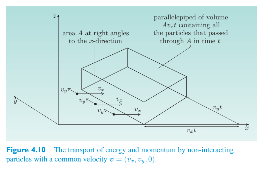
and \(T^{33}\) are all zero because they involve \(v_{z}\), which is zero in this particular case.和 \(T^{33}\) 都为零,因为它们涉及 \(v_z\),在这种特殊情况下 \(v_z\) 为零。
Putting all these results together gives将所有这些结果放在一起得出
The precise form of the energy–momentum tensor will depend on what occupies the region concerned. A particularly simple example to consider is that of a region occupied by a cloud of non-interacting particles, each of mass m. This kind of matter is usually described as dust. For present purposes it’s best to think of the dust cloud as a continuous body of matter that may contain internal currents — rather like a fluid but without any internal pressure. The nature of the dust cloud at any spacetime event in the region of interest can be characterized by the three-velocity v of the flow at the event, and by the value of the cloud’s proper mass density \(\rho\), that is, the density measured by an observer moving with the flow at the event of interest.能量-动量张量的精确形式将取决于相关区域的占据情况。一个特别简单的例子是由非相互作用粒子云占据的区域,每个粒子的质量为 m。这种物质通常被描述为灰尘。就目前的目的而言,最好将尘埃云视为可能包含内部电流的连续物质体——更像是流体,但没有任何内部压力。感兴趣区域中任何时空事件的尘埃云的性质都可以通过该事件处的气流的三速度 v 和云的固有质量密度 \(\rho\) 来表征,即观察者在感兴趣的事件处随气流移动所测量的密度。
Of course, we really want to describe the dust cloud in terms of parameters that have well-known transformation properties under changes of reference frame. This is easy to do: the proper mass density \(\rho\) is a scalar invariant, so it already transforms as simply as possible; the three-velocity v is more complicated, but it can be used to determine a four-velocity \([U^{\mu}]\) = (cγ (v), \(\gamma(v)\) v) (where v = | v | and \(\gamma(v)\) = 1/1 − \(v^{2}\)/\(c^2\)) that transforms as a rank 1 contravariant tensor. The components of the energy–momentum tensor of the dust at any spacetime event can then be written down in a covariant way, in accordance with the rules of tensor algebra, as当然,我们真正想用在参考系变化下具有众所周知的变换特性的参数来描述尘埃云。这很容易做到:适当的质量密度 \(\rho\) 是标量不变量,因此它已经尽可能简单地进行变换;三速度 v 更复杂,但它可用于确定转换为 1 阶逆变张量的四速度 \([U^{\mu}]\) = (cγ (v), \(\gamma(v)\) v)(其中 v = | v | 且 \(\gamma(v)\) = 1/1 − \(v^{2}\)/\(c^2\))。然后,根据张量代数规则,可以以协变的方式写出任意时空事件下的尘埃能量-动量张量的分量,如下
This means that if we choose to use the instantaneous rest frame of the dust at the \([U^{\mu}]\) = (c, 0) and the event in question, then at that event and in that frame, energy–momentum tensor can be represented by the matrix这意味着,如果我们选择使用 \([U^{\mu}]\) = (c, 0) 处尘埃的瞬时静止坐标系和所讨论的事件,那么在该事件和该坐标系中,能量-动量张量可以由矩阵表示
So, in its local instantaneous rest frame, the only non-zero component of the energy–momentum tensor of the dust is \(T^{00}\), which represents the energy density, and that is entirely accounted for by the density of mass–energy in the dust.因此,在其局部瞬时静止坐标系中,尘埃能量-动量张量的唯一非零分量是 \(T^{00}\),它代表能量密度,并且完全由尘埃中的质能密度来解释。
Another simple example of an energy–momentum tensor is that of an ideal fluid. Such a fluid is slightly more complicated than dust, since its nature at any spacetime event is characterized by a mass density \(\rho\), a four-velocity \([U^{\mu}]\) and a pressure p that acts equally in all directions at that point. At an event where the metric is \(g_{\mu\nu}\), the components of the energy–momentum tensor of an ideal fluid are given covariantly by能量-动量张量的另一个简单例子是理想流体。这种流体比尘埃稍微复杂一些,因为它在任何时空事件中的性质都以质量密度 \(\rho\)、四速度 \([U^{\mu}]\) 和在该点在所有方向上作用相同的压力 p 为特征。在度规为 \(g_{\mu\nu}\) 的事件中,理想流体的能量-动量张量的分量由下式协变给出:
If we restrict ourselves to using locally inertial frames with Cartesian coordinates, then at any chosen spacetime event, the metric can be represented by the Minkowski metric, and the components of the energy–momentum tensor will be given by如果我们限制自己使用具有笛卡尔坐标的局部惯性系,那么在任何选定的时空事件中,度规可以用闵可夫斯基度规表示,并且能量-动量张量的分量将由下式给出
If we again take the additional step of considering things from the point of view of an observer using the instantaneous rest frame of the fluid at that point, then, in that frame and at that point, the energy–momentum tensor of the ideal fluid is represented by the matrix如果我们再次采取额外的步骤,使用流体在该点的瞬时静止坐标系从观察者的角度考虑事物,那么,在该坐标系和该点,理想流体的能量-动量张量由矩阵表示
In this case there will generally be thermal effects leading to flows of energy and momentum. However, because we have chosen to use the instantaneous rest frame, those flows will make no net contribution to the flow of energy, so it will still be the case that \(T^{0i}\) = \(T^{i0}\) = 0, and the lack of interactions between the particles will ensure \(T^{ij}=0\) for \(i\ne j\). Consequently, the only non-zero components will be the total energy density \(T^{00}=\rho c^2\) (which will include contributions from the random thermal motion of the particles in the fluid) and the three components \(T^{ii}=p\) for i = 1, 2, 3 (which represent the effect of momentum being transferred with equal magnitude per unit area per unit time in all directions by the thermal motion of the particles).在这种情况下,通常会存在导致能量和动量流动的热效应。然而,由于我们选择使用瞬时静止坐标系,这些流动不会对能量流产生净贡献,因此仍然会出现 \(T^{0i}\) = \(T^{i0}\) = 0 的情况,并且粒子之间缺乏相互作用将确保 \(i\ne j\) 为 \(T^{ij}=0\)。因此,唯一的非零分量将是总能量密度 \(T^{00}=\rho c^2\)(其中包括流体中颗粒的随机热运动的贡献)和 i = 1、2、3 时的三个分量 \(T^{ii}=p\)(其表示通过颗粒热运动在所有方向上每单位面积每单位时间以相等大小传递动量的效果)。
- ● Show that for vanishing pressure (p → 0), the energy–momentum tensor of an证明对于消失压力 (p → 0),能量-动量张量
ideal fluid reduces to that of dust. ❍ For p → 0 we get理想流体可减少为灰尘。 ❍ 对于 p → 0 我们得到
which is Equation 4.23 for the energy–momentum tensor for dust.这是灰尘能量-动量张量的方程 4.23。
- ● Show that the units of pressure (Pa = \(\mathrm{N\,m^{-2}}\)) are equivalent to those of证明压力单位 (Pa = \(\mathrm{N\,m^{-2}}\)) 相当于
energy density (\(\mathrm{J\,m^{-3}}\)), and also equivalent to those used to measure the rate of flow of momentum per unit area.能量密度(\(\mathrm{J\,m^{-3}}\)),也相当于用于测量单位面积动量流速的能量密度。
❍ In SI units, 1 J = 1 N m, so the unit of energy density may be written as❍ 在 SI 单位中,1 J = 1 N m,因此能量密度的单位可写为
\(\mathrm{J\,m^{-3}}\) = N m \(\mathrm{m^{-3}}\) = \(\mathrm{N\,m^{-2}}\) = Pa, which is the unit of pressure. Similarly, the unit of rate of flow of momentum per unit area will be \(\mathrm{kg\,m\,s^{-1}}\) \(\mathrm{m^{-2}}\) \(\mathrm{s^{-1}}\) = \(\mathrm{kg\,m^{-1}\,s^{-2}}\), but 1 N = 1 \(\mathrm{kg\,m\,s^{-2}}\), so the unit of rate of momentum flow per unit area per unit time can be written as\(\mathrm{J\,m^{-3}}\) = N m \(\mathrm{m^{-3}}\) = \(\mathrm{N\,m^{-2}}\) = Pa,这是压力的单位。类似地,单位面积动量流量的单位为 \(\mathrm{kg\,m\,s^{-1}}\) \(\mathrm{m^{-2}}\) \(\mathrm{s^{-1}}\) = \(\mathrm{kg\,m^{-1}\,s^{-2}}\),但 1 N = 1 \(\mathrm{kg\,m\,s^{-2}}\),因此单位时间单位面积动量流量的单位可写为
\(\mathrm{kg\,m^{-1}\,s^{-2}}\) = \(\mathrm{N\,m^{-2}}\) = Pa.kg·m−1·s−2=N·m−2=Pa。
Exercise 4.6 Verify the matrix in Equation 4.27 by练习 4.6 通过以下方式验证方程 4.27 中的矩阵
explicitly evaluating \(T^{00}\), \(T^{0i}\) and \(T^{ij}\) for i, j = 1, 2, 3 from Equation 4.26.根据公式 4.26 显式评估 i、j = 1、2、3 的 \(T^{00}\)、\(T^{0i}\) 和 \(T^{ij}\)。
As a final example of an energy–momentum tensor, we note that in the case of a region of space that contains electric and magnetic fields but no matter (a region occupied by electromagnetic radiation, for example), the components of the energy–momentum tensor are作为能量-动量张量的最后一个例子,我们注意到,在包含电场和磁场但无论如何的空间区域(例如,被电磁辐射占据的区域)的情况下,能量-动量张量的分量为
where F \(\mu\)\(\nu\) is the electromagnetic field tensor that was introduced in Chapter 2. We shall not discuss this energy–momentum tensor in detail, but its existence indicates that in general relativity, electromagnetic radiation alone can be a source of gravitation even though the associated particles (photons) have no mass at all.其中 F \(\mu\)\(\nu\) 是第 2 章中介绍的电磁场张量。我们不会详细讨论这个能量-动量张量,但它的存在表明,在广义相对论中,即使相关粒子(光子)根本没有质量,电磁辐射本身也可以成为引力源。
At this stage it’s useful to recall another result from Chapter 2: in electromagnetism, the conservation of electric charge is represented by the equation of continuity在这个阶段,回顾第二章的另一个结果是有用的:在电磁学中,电荷守恒由连续方程表示
This equation describes how any change in the electric charge density must be balanced by a flow of charge due to electric currents. It is often written more compactly in terms of a three-vector divergence as该方程描述了电荷密度的任何变化必须如何通过电流引起的电荷流来平衡。它通常用三向量散度来写得更紧凑:
or more compactly still, using the current four-vector, by the Lorentz-covariant equation或者更紧凑地,使用当前的四向量,通过洛伦兹协变方程
This suggests that we might expect the conservation of relativistic energy and momentum in a locally inertial frame (where special relativity holds true) to be represented by a relation of the form这表明我们可能期望局部惯性系(狭义相对论成立)中的相对论能量和动量守恒由以下形式的关系表示
and this is indeed the case. The tensor relationship has a free index \(\nu\), so it actually represents four different equations, each of which is similar to the equation of continuity. The first (corresponding to \(\nu\) = 0) relates the rate of change of the energy density \(T^{00}\) to the spatial derivatives of the energy flows \(T^{0i}\) in the 1 -, 2 - and 3 -directions. The other three each relate the rate of change of one of the momentum density terms \(T^{0i}\) to the spatial derivatives of the corresponding momentum flows \(T^{ji}\) for j = 1, 2, 3.事实确实如此。张量关系有一个自由指标 \(\nu\),因此它实际上代表四个不同方程,每个方程都类似于连续性方程。第一个方程(对应 \(\nu=0\))把能量密度 \(T^{00}\) 的变化率同 1、2、3 方向上能量流 \(T^{0i}\) 的空间导数联系起来。其余三个方程则分别把一个动量密度项 \(T^{0i}\) 的变化率同相应动量流 \(T^{ji}\) 的空间导数(\(j=1,2,3\))联系起来。
It also turns out that in arbitrary coordinates and in a spacetime that may be flat or curved, the energy–momentum tensor has the more general property事实证明,在任意坐标和可能是平坦或弯曲的时空中,能量-动量张量具有更一般的性质
This is sometimes described by saying that the covariant divergence of \(T_{\mu\nu}\) is zero. In the absence of gravity, in a flat Minkowski spacetime, this result simply allows us to describe the conservation of energy and momentum using general coordinates. However, if the spacetime is curved, then it turns out that Equation 4.30 does not generally describe the conservation of energy and momentum for the contents of spacetime. And that’s a good thing, because in the presence of gravitation (i.e. curvature), the conservation of energy is not expected to apply to matter and radiation alone — we also have to take the gravitational energy into account, and that is not included in the energy–momentum tensor. We shall return to the significance of the covariant divergence in curved spacetime later; for the moment we just need to emphasize the following.有时用 \(T_{\mu\nu}\) 的协变散度为零来描述这一点。在没有引力的情况下,在平坦的闵可夫斯基时空中,这个结果让我们能够使用通用坐标来描述能量和动量守恒。然而,如果时空是弯曲的,那么方程 4.30 并不能概括地描述时空内容的能量和动量守恒。这是一件好事,因为在存在引力(即曲率)的情况下,能量守恒预计不仅仅适用于物质和辐射——我们还必须考虑引力能,而这不包括在能量-动量张量中。稍后我们将回到弯曲时空中协变散度的意义;目前我们只需要强调以下几点。
The energy–momentum tensor能量-动量张量
The energy–momentum tensor \(T_{\mu\nu}\) describes the distribution and flow of energy and momentum due to the presence and motion of matter and radiation in a region of spacetime. It is a rank 2, symmetric tensor with ten independent components. At any event in the region of interest, its components describe the energy density, the flow of energy in various directions, divided by c (or, equivalently, the density of the corresponding momentum component, multiplied by c), and the flow of the various momentum components in the various directions.能量-动量张量 \(T_{\mu\nu}\) 描述了由于时空区域中物质和辐射的存在和运动而导致的能量和动量的分布和流动。它是一个具有 10 个独立分量的 2 阶对称张量。在感兴趣区域中的任何情况下,其分量描述能量密度、各个方向上的能量流除以 c(或者等效地,相应动量分量的密度乘以 c)以及各个方向上各个动量分量的流。
For pressure-free dust, the components of the energy–momentum tensor are given by对于无压灰尘,能量-动量张量的分量由下式给出
for an ideal fluid,对于理想流体,
and for electromagnetic fields,对于电磁场,
An important general property of the energy–momentum tensor is that its covariant divergence is zero; that is,能量-动量张量的一个重要的一般性质是它的协变散度为零;那是,
4.2.2 The Einstein tensor4.2.2 爱因斯坦张量
The equivalence principle led Einstein to propose that gravity should be regarded not as a force in the conventional sense, but as a manifestation of the curvature of spacetime. Einstein was therefore looking for a geometric theory of gravity, so he needed to find a geometric object that could be related to the energy–momentum tensor. Clearly, he needed a rank 2 tensor involving the components of the metric tensor. However, from the example of the electromagnetic field equations, or even from Newtonian gravity formulated as a field theory and based on Poisson’s equation, we should expect the final equations to be differential equations, so the metric should enter through its derivatives. We might also expect that the required geometric tensor will be symmetric and will have a vanishing covariant divergence.等效原理促使爱因斯坦提出,引力不应被视为传统意义上的力,而应被视为时空曲率的表现。因此,爱因斯坦正在寻找引力的几何理论,因此他需要找到一个可以与能量-动量张量相关的几何物体。显然,他需要一个包含度规张量分量的 2 阶张量。然而,从电磁场方程的例子来看,甚至从作为场论形式表达的牛顿引力和基于泊松方程的例子来看,我们应该期望最终的方程是微分方程,因此度规应该通过其导数进入。我们还可能期望所需的几何张量是对称的并且协变散度消失。
Even with so many clues, it took Einstein some time to find the appropriate tensor quantity. What he eventually arrived at involved contractions of the Riemann curvature tensor that was introduced in Chapter 3. Here is the full form of the Riemann tensor for a four-dimensional spacetime:即使有这么多线索,爱因斯坦还是花了一些时间才找到合适的张量。他最终得出的结论涉及第 3 章中介绍的黎曼曲率张量的收缩。以下是四维时空黎曼张量的完整形式:
δ αβ, which are defined in As you can see, it involves the connection coefficients Γ terms of the metric and its derivatives byδ αβ,如您所见,它涉及度规及其导数的联络系数 Γ 项
You will recall from Chapter 3 that the vanishing of all components of the Riemann tensor is the necessary and sufficient condition for a spacetime to be flat.你会记得在第三章中,黎曼张量所有分量的消失是时空平坦的充分必要条件。
The Riemann tensor has four indices, each of which can take four values (in four-dimensional spacetime), so it has 4 4 = 256 components. However, the tensor has various symmetries, so there are just 20 independent components.黎曼张量有四个索引,每个索引可以取四个值(在四维时空中),因此它有 4 4 = 256 个分量。然而,张量具有各种对称性,因此只有 20 个独立分量。
Although the Riemann tensor is fundamental to the study of curved spaces, there are two other tensors that have been found to be very useful. If we contract the first and last indices on the Riemann tensor, then we get a new rank 2 tensor with components尽管黎曼张量是弯曲空间研究的基础,但还有其他两个张量被发现非常有用。如果我们收缩黎曼张量的第一个和最后一个索引,那么我们会得到一个带有分量的新的 2 阶张量
which is known as the Ricci tensor. It follows from the definition of the Riemann tensor that the Ricci tensor is symmetric with respect to interchanging its indices, i.e. R αβ = R βα. Further, contracting the indices on the Ricci tensor gives这就是所谓的里奇张量。根据黎曼张量的定义可知,里奇张量在交换其指数方面是对称的,即 R αβ = R βα。此外,收缩 Ricci 张量的指数给出
which is known as the curvature scalar (or sometimes the Ricci scalar). Note that all of these curvature-related quantities are ultimately expressed in terms of the components of the metric tensor \(g_{\mu\nu}\) and their derivatives.这称为曲率标量(有时称为 Ricci 标量)。请注意,所有这些与曲率相关的量最终都以度规张量 \(g_{\mu\nu}\) 的分量及其导数来表示。
The quantity that Einstein found to be a basic ingredient of general relativity is defined in terms of the Ricci tensor and the curvature scalar. It is called the Einstein tensor and its components are given by the following equation.爱因斯坦发现广义相对论基本成分的量是用里奇张量和曲率标量定义的。它称为爱因斯坦张量,其分量由以下方程给出。
The Einstein tensor爱因斯坦张量
Since both R \(\mu\)\(\nu\) and \(g_{\mu\nu}\) are symmetric, it follows that G \(\mu\)\(\nu\) must also be symmetric. This means that only 10 of its 16 components will be independent, just like the energy–momentum tensor. Moreover, it! can be shown that B the \(\mu\) ∇ \(\mu\) G \(\mu\)\(\nu\) = 0, again covariant divergence of the Einstein tensor vanishes just like the energy–momentum tensor.由于 R \(\mu\)\(\nu\) 和 \(g_{\mu\nu}\) 都是对称的,因此 G \(\mu\)\(\nu\) 也必须是对称的。这意味着它的 16 个分量中只有 10 个是独立的,就像能量-动量张量一样。更何况,它!可以证明 B \(\mu\) ∇ \(\mu\) G \(\mu\)\(\nu\) = 0,爱因斯坦张量的协变散度再次消失,就像能量-动量张量一样。
We are now in a position to introduce Einstein’s field equations, the mathematical relations that are at the core of general relativity.我们现在可以介绍爱因斯坦的场方程,这是广义相对论核心的数学关系。
4.3 Einstein’s field equations and geodesic motion4.3 爱因斯坦场方程和测地运动
The central ideas of general relativity were famously summed up by the American physicist John Wheeler:美国物理学家约翰·惠勒对广义相对论的中心思想做出了著名的总结:
Matter tells space how to curve. Space tells matter how to move.物质告诉空间如何弯曲。空间告诉物质如何运动。
This is very memorable (and worth remembering!), though not completely accurate. (You should already be asking yourself: ‘Doesn’t he mean spacetime rather than space, and doesn’t he mean matter and radiation rather than matter?’) Unpacking Wheeler’s quote somewhat, to be more accurate, we can say that the central physical ideas of general relativity are that the energy and momentum in a region of spacetime determine the geometry of spacetime in that region. The spacetime geometry then determines a special class of spacetime pathways — the geodesics. Moving under the influence of gravity alone, massive particles travel along time-like geodesics (where \(ds^2\) > 0), while light rays follow null geodesics (with \(ds^2\) = 0). Thus the distribution of energy and momentum in a region determines the motion of freely falling matter and radiation in that region.这是非常令人难忘的(并且值得记住!),尽管并不完全准确。(你应该已经问自己:“他不是指的是时空而不是空间,他不是指的是物质和辐射而不是物质吗?”)稍微解释一下惠勒的引言,更准确地说,我们可以说广义相对论的核心物理思想是时空区域中的能量和动量决定了该区域中时空的几何形状。然后,时空几何决定了一类特殊的时空路径——测地线。仅在引力影响下移动,大质量粒子沿着类时测地线(其中 \(ds^2\) > 0)行进,而光线则遵循零测地线(其中 \(ds^2\) = 0)。因此,一个区域中能量和动量的分布决定了该区域中自由落体物质和辐射的运动。
Another helpful but overly simple view is that in Newtonian gravitation, matter tells matter how to move, with the gravitational force playing the role of intermediary. This can be contrasted with general relativity where energy and momentum tell matter and radiation how to move, with spacetime geometry playing the role of intermediary.另一个有用但过于简单的观点是,在牛顿引力中,物质告诉物质如何运动,而引力则扮演中介的角色。这可以与广义相对论形成对比,广义相对论中能量和动量告诉物质和辐射如何移动,而时空几何则扮演中介的角色。
The rest of this section is devoted to spelling out these ideas with greater accuracy and improved precision.本节的其余部分致力于以更高的准确性和更高的精度阐明这些想法。
4.3.1 The Einstein field equations4.3.1 爱因斯坦场方程
As we have seen, Einstein’s objective became the formulation of a ‘geometric’ theory of gravity that would naturally act on all kinds of matter in the same way. He identified the energy–momentum tensor as an important quantity for describing the ‘sources’ of gravitation, and found another symmetric rank 2 tensor, the Einstein tensor, containing derivatives of the metric coefficients \(g_{\mu\nu}\), tensor \(T_{\mu\nu}\) and the that he could relate to it. Both the energy–momentum Einstein tensor [G \(\mu\)\(\nu\)] have zero covariant divergence, so it is natural to suggest that the two tensors are proportional. This led Einstein to propose what are now called the Einstein field equations, which are usually written as in terms of tensor components as follows.正如我们所看到的,爱因斯坦的目标变成了引力的“几何”理论的表述,该理论自然会以相同的方式作用于所有种类的物质。他认为能量-动量张量是描述引力“来源”的重要量,并发现了另一个对称的 2 阶张量,即爱因斯坦张量,其中包含度规系数 \(g_{\mu\nu}\)、张量 \(T_{\mu\nu}\) 的导数以及他可以与之关联的。能量-动量爱因斯坦张量 [G \(\mu\)\(\nu\)] 的协变散度为零,因此很自然地认为这两个张量成比例。这导致爱因斯坦提出了现在所谓的爱因斯坦场方程,该方程通常用张量分量写成如下。
The Einstein field equations爱因斯坦场方程
Here \(\kappa\) is a constant, sometimes called the Einstein constant. We shall show later that requiring the consistency of general relativity and Newtonian gravitation forces us to set \(\kappa = 8\pi G/c^4\).这里 \(\kappa\) 是一个常数,有时称为爱因斯坦常数。稍后我们将证明,要求广义相对论和牛顿引力的一致性迫使我们设置 \(\kappa = 8\pi G/c^4\)。
The Einstein field equations are the fundamental field equations of general relativity, analogous to the Poisson equation in Newtonian gravitation. They are the feature of general relativity that Wheeler was referring to when he said (rather loosely) ‘matter tells space how to curve’. The Einstein field equations have two free indices, \(\mu\) and \(\nu\), so they actually represent a set of 16 equations, though due to symmetries only 10 of them are independent. They are usually regarded as differential equations for the 10 independent metric tensor components \(g_{\mu\nu}\). But they are generally very complicated.爱因斯坦场方程是广义相对论的基本场方程,类似于牛顿引力中的泊松方程。它们是惠勒(相当宽松地)“物质告诉空间如何弯曲”时所指的广义相对论的特征。爱因斯坦场方程有两个自由索引,\(\mu\) 和 \(\nu\),因此它们实际上代表一组 16 个方程,但由于对称性,其中只有 10 个方程是独立的。它们通常被视为 10 个独立度规张量分量 \(g_{\mu\nu}\) 的微分方程。但它们通常非常复杂。
The reason for the complication is not hard to see. The Ricci tensor and the curvature scalar involve combinations of components of the Riemann tensor. Its coefficients Γ \(\mu\) αβ, components R \(\mu\) \(\nu\)αβ are defined in terms of the connection which are in turn defined in terms of the metric tensor components \(g_{\mu\nu}\) and the components of its inverse \(g_{\mu\nu}\). The way in which the connection coefficients appear in R \(\mu\) \(\nu\)αβ means that the Riemann tensor involves second-order derivatives of the metric coefficients with respect to the spacetime coordinates. However, because the connection coefficients involve both the metric tensor and its inverse, the Einstein field equations are non-linear in \(g_{\mu\nu}\). (An equation is said to be non-linear in a variable y if replacing y by αy throughout the equation does not produce an equation that is equivalent to the original equation multiplied by \(\alpha\).) It is the non-linearity that makes the Einstein field equations particularly difficult to solve.造成并发症的原因不难看出。里奇张量和曲率标量涉及黎曼张量分量的组合。它的系数 Γ \(\mu\) αβ,分量 R \(\mu\) \(\nu\)αβ 根据联络定义,而联络又根据度规张量分量 \(g_{\mu\nu}\) 及其逆 \(g_{\mu\nu}\) 的分量定义。R \(\mu\) \(\nu\)αβ 中联络系数的出现方式意味着黎曼张量涉及度规系数相对于时空坐标的二阶导数。然而,由于联络系数同时涉及度规张量及其逆,因此 \(g_{\mu\nu}\) 中的爱因斯坦场方程是非线性的。(如果在整个方程中用 αy 替换 y 不能产生等于原始方程乘以 \(\alpha\) 的方程,则称该方程在变量 y 中是非线性的。)正是这种非线性使得爱因斯坦场方程特别难以求解。
Solving the Einstein field equations means finding the metric tensor \(g_{\mu\nu}\) that corresponds to a given energy–momentum tensor \(T_{\mu\nu}\). As you saw in Chapter 3, the metric tensor, once it is known, will determine the connection coefficients, the curvature tensor, the geodesic pathways and all the other geometric features of the spacetime that it describes. Given that gravitation is ‘built in’ to the geometry of spacetime in general relativity, the metric tensor that corresponds to a given set of source terms (i.e. a given energy–momentum tensor) is the gravitational field, even though it is not the ‘force per unit mass’ of the Newtonian gravitational field.求解爱因斯坦场方程意味着找到对应于给定能量-动量张量 \(T_{\mu\nu}\) 的度规张量 \(g_{\mu\nu}\)。正如您在第 3 章中看到的,度规张量一旦已知,将确定联络系数、曲率张量、测地线路径以及它所描述的时空的所有其他几何特征。鉴于引力是广义相对论中时空几何的“内置”,对应于给定源项集(即给定能量-动量张量)的度规张量就是引力场,尽管它不是牛顿引力场的“每单位质量的力”。
The act of solving the Einstein field equations might sound straightforward, but the ten independent field equations form a set of simultaneous, non-linear, second-order partial differential equations and, depending on the energy–momentum tensor, the task of finding a solution varies between difficult and impossible. In fact, it is remarkable that the first (and probably most important) exact non-trivial solution was announced very soon after Einstein first proposed his equations. We shall describe that solution in the next chapter.求解爱因斯坦场方程的行为可能听起来很简单,但十个独立的场方程形成了一组联立、非线性、二阶偏微分方程,并且根据能量-动量张量的不同,找到解决方案的任务有时是困难的,有时是不可能的。事实上,值得注意的是,在爱因斯坦首次提出他的方程之后不久,第一个(也可能是最重要的)精确的非平凡解就被宣布了。我们将在下一章中描述该解决方案。
In addition to various numerical procedures for finding solutions to the field equations, there are three different ways to approach the search for solutions.除了寻找场方程解的各种数值程序之外,还可以采用三种不同的方法来寻找解。
1. As already suggested, we could specify the energy–momentum tensor and1. 正如已经建议的,我们可以指定能量-动量张量和
then work very hard to solve for the metric components \(g_{\mu\nu}\). This approach has actually been very successful for some energy–momentum tensors.然后非常努力地求解度规分量 \(g_{\mu\nu}\)。这种方法实际上对于某些能量-动量张量非常成功。
2. We could specify the metric tensor and then work out the energy–momentum2.我们可以指定度规张量,然后计算出能量-动量
tensor. This is generally easier since it is more straightforward to differentiate a function than to solve a non-linear partial differential equation. However, it usually turns out that the resulting energy–momentum tensor is non-physical, so this approach is not as useful as might be hoped.张量。这通常更容易,因为微分函数比求解非线性偏微分方程更直接。然而,通常结果表明所得到的能量-动量张量是非物理的,因此这种方法并不像希望的那样有用。
3. We could try to partly determine both the metric tensor and the3. 我们可以尝试部分确定度规张量和
energy–momentum tensor directly from the physics of a particular situation and then use the field equations as constraints to complete the determination of \(g_{\mu\nu}\) and \(T_{\mu\nu}\). This sometimes yields useful results.直接从特定情况的物理场中获取能量-动量张量,然后使用场方程作为约束来完成 \(g_{\mu\nu}\) 和 \(T_{\mu\nu}\) 的确定。这有时会产生有用的结果。
In any case, a significant part of the discovery of any new solution of the Einstein field equations is to check that the solution really is new, and not merely an old solution expressed in a different coordinate system. This is an interesting problem but its consideration would take us well beyond the limits of this book.无论如何,发现爱因斯坦场方程的任何新解的一个重要部分是检查该解是否确实是新的,而不仅仅是在不同坐标系中表达的旧解。这是一个有趣的问题,但对它的考虑将远远超出本书的范围。
- ● Taking the metric tensor components \(g_{\mu\nu}\) to be dimensionless quantities将度规张量分量 \(g_{\mu\nu}\) 视为无量纲量
(i.e. pure numbers), show that the connection coefficients Γ \(\lambda\) \(\mu\)\(\nu\) can be expressed in units of \(\mathrm{m^{-1}}\), while the Ricci tensor [R \(\mu\)\(\nu\)] and the curvature scalar R can both be expressed in units of \(\mathrm{m^{-2}}\). Combine this with your knowledge of the appropriate units for \(T_{\mu\nu}\) to show that 8 πG/\(c^4\) has the right units to be the Einstein constant \(\kappa\).(即纯数),表明联络系数 Γ \(\lambda\) \(\mu\)\(\nu\) 可以用 \(\mathrm{m^{-1}}\) 为单位表示,而 Ricci 张量 [R \(\mu\)\(\nu\)] 和曲率标量 R 都可以用 \(\mathrm{m^{-2}}\) 为单位表示。将其与您对 \(T_{\mu\nu}\) 的适当单位的了解相结合,以证明8 πG/\(c^4\) 的正确单位是爱因斯坦常数 \(\kappa\)。
❍ Since \(g_{\mu\nu}\) is dimensionless, it follows from❍ 由于 \(g_{\mu\nu}\) 是无量纲的,因此可以得出
that Γ \(\lambda\) \(\mu\)\(\nu\) can be expressed in units of \(\mathrm{m^{-1}}\). It then follows from则 Γ \(\lambda\) \(\mu\)\(\nu\) 可以用 \(\mathrm{m^{-1}}\) 为单位表示。然后可得
that R δ αβγ can be expressed in units of \(\mathrm{m^{-2}}\), but [R \(\mu\)\(\nu\)] and R are sums of components of R δ αβγ, so they too can be expressed in units of \(\mathrm{m^{-2}}\). With this in mind and recalling that the components of the energy–momentum tensor can be expressed in units of \(\mathrm{J\,m^{-3}}\) = \(\mathrm{kg\,m^{-1}\,s^{-2}}\), it can be seen that suitable units for \(\kappa\) are (1/\(m^{2}\))(1/(\(\mathrm{kg\,m^{-1}\,s^{-2}}\))) = \(\mathrm{kg^{-1}\,m^{-1}\,s^2}\), and the units of 8 πG/\(c^4\) are indeed N \(m^{2}\) kg − 2 s 4 m − 4 = \(\mathrm{kg^{-1}\,m^{-1}\,s^2}\).可知 R δ αβγ 可以用 \(\mathrm{m^{-2}}\) 为单位表示,但 [R \(\mu\)\(\nu\)] 和 R 是 R δ αβγ 各分量的和,因此它们也可以用 \(\mathrm{m^{-2}}\) 为单位表示。考虑到这一点,回想一下能量-动量张量的分量可以用 \(\mathrm{J\,m^{-3}}\) = \(\mathrm{kg\,m^{-1}\,s^{-2}}\) 的单位表示,可以看出,\(\kappa\) 的合适单位为 (1/m 2)(1/(\(\mathrm{kg\,m^{-1}\,s^{-2}}\))) = \(\mathrm{kg^{-1}\,m^{-1}\,s^2}\),而 8 πG/\(c^4\) 的单位为事实上,N m 2 kg − 2 s 4 m − 4 = \(\mathrm{kg^{-1}\,m^{-1}\,s^2}\)。
Exercise 4.7 Show that Equation 4.34 can also be written练习 4.7 证明方程 4.34 也可以写成
as作为
where T ≡ \(\mu\) T \(\mu\) \(\mu\). (Hint: Multiply the Einstein field equations by \(g_{\mu\nu}\), and contract.)其中 T ≠ \(\mu\) T \(\mu\) \(\mu\)。 (提示:将爱因斯坦场方程乘以 \(g_{\mu\nu}\),然后收缩。)
In some regions of spacetime, it may be that \(T_{\mu\nu}\) = 0. In such regions, spacetime is said to be empty. Equation 4.35 shows that in such a region, the Einstein field equations may be written as在时空的某些区域中,\(T_{\mu\nu}\) = 0。在这些区域中,时空被称为空的。方程 4.35 显示,在这样的区域中,爱因斯坦场方程可写为
Note that this does not necessarily mean that spacetime in the region is flat. The necessary and sufficient condition for flatness is that the components of the Riemann tensor should vanish at all events in the region, but that tensor has 20 components while the Ricci tensor has only 10. The vanishing of R \(\mu\)\(\nu\) in some, nor, therefore, does it region does not necessarily imply the vanishing of R \(\mu\) \(\nu\)αβ \(T_{\mu\nu}\) = 0 does indicate imply that \(g_{\mu\nu}\) describes a flat spacetime. However, setting that there is no matter or radiation in the region concerned, so solutions of Equation 4.36 are said to be vacuum solutions of the field equations. The study of vacuum solutions is an important sub-field of general relativity.请注意,这并不一定意味着该区域的时空是平坦的。平坦的充分必要条件是黎曼张量的分量在该区域的所有事件中都应该消失,但该张量有 20 个分量,而里奇张量只有 10 个。R \(\mu\)\(\nu\) 在某些区域的消失,因此,它并不一定意味着 R \(\mu\) \(\nu\)αβ \(T_{\mu\nu}\) = 0 的消失确实表明暗示 \(g_{\mu\nu}\) 描述了平坦的时空。然而,假设相关区域不存在物质或辐射,因此方程 4.36 的解被称为场方程的真空解。真空解的研究是广义相对论的一个重要子领域。
4.3.2 Geodesic motion4.3.2 测地运动
Einstein completed his long search for the field equations in 1915 and announced the basic principles of general relativity in a talk at the Prussian Academy of Sciences in Berlin in November 1915. The details of the theory were published in爱因斯坦于 1915 年完成了对场方程的长期探索,并于 1915 年 11 月在柏林普鲁士科学院的一次演讲中宣布了广义相对论的基本原理。该理论的详细信息发表于
1916. At that time Einstein clearly understood that in addition1916年。当时爱因斯坦清楚地认识到,除了
to using the field equations to find the spacetime metric, the theory also required that the metric should be used to determine the geodesics of the spacetime via the geodesic equations. These were introduced in Chapter 3. For a four-dimensional spacetime with metric tensor \(g_{\mu\nu}\), they take the form为了使用场方程找到时空度规,该理论还要求使用该度规通过测地线方程确定时空的测地线。这些已在第 3 章中介绍。对于具有度规张量 \(g_{\mu\nu}\) 的四维时空,它们采用以下形式
where \(\lambda\) is an affine parameter and, as usual,其中 \(\lambda\) 是仿射参数,并且像往常一样,
The functions x \(\rho\) (\(\lambda\)) that satisfy the geodesic equation describe parameterized curves through spacetime that represent the most direct routes between events. (A tangent to such a curve, parallel transported along the curve, remains a tangent.) So these geodesic curves are the analogues of straight lines in a curved space.满足测地线方程的函数 x \(\rho\) (\(\lambda\)) 描述了时空参数化曲线,代表事件之间最直接的路线。 (这样一条曲线的切线,沿曲线平行传输,仍然是切线。)因此,这些测地曲线类似于弯曲空间中的直线。
You will recall from Chapter 3 that given a curve specified by the coordinate functions x \(\rho\) (\(\lambda\)), the components of the tangent vector to the curve at the point你会记得在第 3 章中,给定一条由坐标函数 x \(\rho\) (\(\lambda\)) 指定的曲线,该点处曲线的切向量的分量
We can associate a sort, of ‘length’ with this vector (actually called its norm) defined by the quantity \(\alpha\),\(\beta\) t \(\alpha\) t \(\beta\). In the case of an affinely parameterized geodesic, where the tangent vector remains a tangent vector under parallel transport, this norm will be the same at all points. Thus we can separate the geodesics into three distinct classes:我们可以将“长度”的类别与由数量 \(\alpha\),\(\beta\) t \(\alpha\) t \(\beta\) 定义的向量(实际上称为其范数)相关联。在仿射参数化测地线的情况下,切向量在平行传输下仍然是切向量,该范数在所有点上都是相同的。因此,我们可以将测地线分为三个不同的类别:
- • time-like geodesics, where the tangent vector always has positive norm类时间测地线,其中切向量始终具有正范数
- • null geodesics, where the tangent vector always has zero norm零测地线,其中切向量始终具有零范数
- • space-like geodesics, where the tangent vector always has negative norm.类空间测地线,其中切向量始终具有负范数。
In the case of the time-like and space-like geodesics, the line element separating neighbouring points on the geodesic, given by在类时间和类空间测地线的情况下,分隔测地线上相邻点的线元素由下式给出
will always be non-zero, and we can use the square root of its magnitude | \(ds^2\) | 1/2 to define a distance element that we can use when parameterizing the geodesic. These geodesics are collectively described as non-null geodesics. In the contrasting case of a null geodesic, the line element separating neighbouring points will always be zero, so there is no possibility of using the ‘distance’ along the curve as the parameter \(\lambda\) in that case, even though it can still be parameterized in other ways.总是非零,我们可以使用其大小 | 的平方根d s 2 | 1/2 定义我们在参数化测地线时可以使用的距离元素。这些测地线统称为非零测地线。在零测地线的对比情况下,分隔相邻点的线元素将始终为零,因此在这种情况下不可能使用沿曲线的“距离”作为参数 \(\lambda\),即使它仍然可以通过其他方式参数化。
What is the significance of all this for general relativity and gravity? It is contained in the following assertion.这一切对于广义相对论和引力有何意义?它包含在以下断言中。
The principle of geodesic motion测地运动原理
In general relativity, the time-like geodesics of a spacetime represent the possible world-lines of massive particles falling freely under the influence of gravity alone. And, similarly, the null geodesics of a spacetime represent the possible world-lines of massless particles moving under the influence of gravity alone.在广义相对论中,时空的类时间测地线代表了仅在引力影响下自由落体的大质量粒子的可能世界线。同样,时空的零测地线代表了仅在引力影响下运动的无质量粒子的可能世界线。
This is what Wheeler was referring to when he said (somewhat loosely) ‘space tells matter how to move’.这就是惠勒(有点宽松)所说的“空间告诉物质如何移动”时所指的内容。
The principle implies that, in the absence of any non-gravitational effects, the path through spacetime followed by a planet as it orbits a star will be a time-like geodesic of the spacetime that surrounds the star. And, similarly, the spacetime pathway of a flash of light leaving the star will be a null geodesic of that spacetime.该原理意味着,在没有任何非引力效应的情况下,行星绕恒星运行时所遵循的时空路径将是围绕恒星的时空的类时间测地线。同样,离开恒星的闪光的时空路径将是该时空的零测地线。
In 1915–16, Einstein thought that the principle of geodesic motion was a separate postulate that was needed alongside the field equations to make general relativity a complete theory of gravity. However, later work by Einstein and others eventually showed that the geodesic motion of freely falling matter and radiation is actually predicted by the field equations through the requirement that1915-16 年,爱因斯坦认为测地运动原理是一个单独的假设,需要与场方程一起使广义相对论成为完整的引力理论。然而,爱因斯坦和其他人后来的工作最终表明,自由落体物质和辐射的测地运动实际上是通过场方程通过以下要求来预测的:
It is a remarkable feature of general relativity that it predicts the equations of motion of the matter and radiation that is also the source of gravitation. This is another aspect of the non-linearity of the theory.广义相对论的一个显着特征是它预测了物质和辐射的运动方程,辐射也是万有引力的来源。这是该理论非线性的另一个方面。
4.3.3 The Newtonian limit of Einstein’s4.3.3 爱因斯坦的牛顿极限
field equations场方程
One of the guiding principles in Einstein’s search for a geometric theory of gravity was what we have called the principle of consistency, so it is important to show that under appropriate circumstances, the Einstein field equations are consistent with Poisson’s equation爱因斯坦寻找引力几何理论的指导原则之一就是我们所说的一致性原理,因此重要的是要证明在适当的情况下,爱因斯坦场方程与泊松方程是一致的
The ‘appropriate circumstances’ that define what is usually referred to as the Newtonian limit of general relativity suppose that the gravitational effects are weak and that any motions are sufficiently slow to be considered ‘non-relativistic’. Also, remember that Newtonian gravitation concerns the movement of only matter, not radiation.定义通常所说的广义相对论牛顿极限的“适当情况”假设引力效应很弱,并且任何运动都足够慢,可以被视为“非相对论”。另外,请记住,牛顿引力只涉及物质的运动,而不涉及辐射。
The assumption that gravitational effects are weak allows us to assume that the metric coefficients are close to those of the Minkowski引力效应较弱的假设使我们可以假设度规系数接近闵可夫斯基的系数
where | h \(\mu\)\(\nu\) | (1, and we can choose to work to first order in h \(\mu\)\(\nu\). We can also suppose that the metric is not changing significantly with time, so h \(\mu\)\(\nu\) is not a function of time.哪里 | h \(\mu\)\(\nu\) | (1,我们可以选择对 h \(\mu\)\(\nu\) 中的一阶进行处理。我们还可以假设该度规不会随时间显着变化,因此 h \(\mu\)\(\nu\) 不是时间的函数。
Now, if we consider the simple, case of a region filled with dust, for which T = \(\rho\) U U and T = T \(\mu\) = ρc 2, we can see that the Einstein field equations given in Equation 4.35 take the form现在,如果我们考虑一个充满灰尘的区域的简单情况,其中 T = \(\rho\) U U 且 T = T \(\mu\) = ρc 2,我们可以看到方程 4.35 中给出的爱因斯坦场方程采用以下形式
Substituting our simplified form of the metric gives替换我们的度规的简化形式给出
Examining the \(R^{00}\) term, and remembering that speeds检查 \(R^{00}\) 术语,并记住速度
However, in the same limit, it can be shown from the definition of the Ricci tensor that然而,在同样的极限下,由 Ricci 张量的定义可以看出:
and from the definition of the connection coefficient that and consequently并根据联络系数的定义得出
Equating the two expressions that we now have for \(R^{00}\), we see that in the Newtonian limit,把现在得到的 \(R^{00}\) 的两个表达式相等,就可看到在牛顿极限下,
and so所以
This result already looks something like Poisson’s equation, but to really make the link we need to know how \(h_{00}\) is related to the Newtonian gravitational potential \(\Phi\). This relationship can be determined from the geodesic equation of motion of a particle. We shall not go through the detailed argument, but it turns out that in the Newtonian limit, \(\Phi=h_{00}c^2/2\). Using this identification, we see that in the Newtonian limit, general relativity predicts that这个结果看起来已经有点像泊松方程,但若要真正建立联系,我们需要知道 \(h_{00}\) 与牛顿引力势 \(\Phi\) 的关系。这种关系可以从粒子的测地线运动方程确定。我们不详细展开论证,但结果表明,在牛顿极限下 \(\Phi=h_{00}c^2/2\)。利用这一辨识,可以看到在牛顿极限下,广义相对论预言
which approximates Poisson’s equation近似泊松方程
provided that we identify \(\kappa = 8\pi G/c^4\).前提是我们识别 \(\kappa = 8\pi G/c^4\)。
Thus general relativity agrees with Newtonian gravitation in the limit of low speeds and weak fields, provided that \(\kappa = 8\pi G/c^4\).因此,广义相对论在低速弱场的极限下与牛顿引力一致,只要 \(\kappa = 8\pi G/c^4\) 即可。
4.3.4 The cosmological constant4.3.4 宇宙学常数
We shall end this discussion of the field equations with a brief introduction to a topic that will be discussed at greater length in the final chapter. It concerns a modification to the field equations that Einstein proposed but later described as ‘the greatest blunder of my life’, though it is now regarded as a very important aspect of general relativity.我们将通过简要介绍一个主题来结束对场方程的讨论,该主题将在最后一章进行更详细的讨论。它涉及爱因斯坦提出的场方程的修改,但后来被描述为“我一生中最大的错误”,尽管它现在被认为是广义相对论的一个非常重要的方面。
The field equations that have been presented in this chapter are those that Einstein presented in 1916 and on which he based a number of astronomical predictions that were used to test general relativity. (These tests will be discussed later.) However, in 1917 he turned his attention to cosmology — the study of the Universe — and realized that he had omitted a term that was mathematically justified and might be important. Including this additional cosmological term, the modified field equations take the form本章中介绍的场方程是爱因斯坦在 1916 年提出的场方程,他基于这些方程做出了许多用于检验广义相对论的天文学预测。 (这些测试将在稍后讨论。)然而,1917 年,他将注意力转向宇宙学——对宇宙的研究——并意识到他省略了一个在数学上合理且可能很重要的术语。包括这个附加的宇宙学项,修正后的场方程采用以下形式
where \(\Lambda\) represents a new universal constant of Nature known as the cosmological constant. Einstein’s original motivation for introducing this constant was that at the time, the Universe was thought to be static (i.e. neither expanding nor contracting), and he found that a non-zero value of \(\Lambda\) could lead to static solutions of the field equations (although they later turned out to be unstable). In the其中 \(\Lambda\) 代表一个新的自然通用常数,称为宇宙学常数。爱因斯坦引入这个常数的最初动机是,当时宇宙被认为是静态的(即既不膨胀也不收缩),他发现 \(\Lambda\) 的非零值可以导致场方程的静态解(尽管后来证明它们是不稳定的)。在
Newtonian limit, a positive value of \(\Lambda\) provides a repulsive effect that can counterbalance the usual gravitational attraction. It was the subsequent discovery that the Universe was in fact expanding that prompted Einstein to make his comment about the cosmological constant being his ‘greatest blunder’.牛顿极限,\(\Lambda\) 的正值提供排斥效应,可以抵消通常的万有引力。正是随后发现宇宙实际上正在膨胀,促使爱因斯坦发表了关于宇宙学常数是他“最大的错误”的评论。
Ironically, observational evidence now favours the view that the Universe is not only expanding, but is doing so at an accelerating rate. The cosmological constant, a new fundamental constant, is one way of explaining this. But there are others.讽刺的是,现在的观测证据支持这样的观点:宇宙不仅在膨胀,而且还在加速膨胀。宇宙学常数,一个新的基本常数,是解释这一点的一种方式。但还有其他的。
From a mathematical point of view, we can transfer the cosmological term to the right-hand side of the field equations, giving从数学的角度来看,我们可以将宇宙项转移到场方程的右侧,给出
The cosmological term now begins to look like some additional contribution to the energy and momentum. We can further this impression by regarding the − (\(\Lambda\)/\(\kappa\)) \(g_{\mu\nu}\) term as arising from a new part of the energy–momentum tensor that we represent by \(T_{\mu\nu}\). The modified field equations then take the form宇宙学术语现在开始看起来像是对能量和动量的一些额外贡献。我们可以通过将 - (\(\Lambda\)/\(\kappa\)) \(g_{\mu\nu}\) 项视为源自我们用 \(T_{\mu\nu}\) 表示的能量-动量张量的新部分来进一步加深这种印象。修正后的场方程采用以下形式
If we take the additional step of treating the new contribution as if it comes from an ideal fluid with density \(\rho_{\Lambda}\) and pressure \(p_{\Lambda}\), then we can use Equation 4.25 to write如果我们采取额外的步骤,将新的贡献视为来自密度为 \(\rho_{\Lambda}\) 且压力为 \(p_{\Lambda}\) 的理想流体,那么我们可以使用方程 4.25 写出
where we say that \(\rho_{\Lambda}\) \(c^2\) represents the density of dark energy and \(p_{\Lambda}\) is the pressure due to dark energy. We can ensure that其中 \(\rho_{\Lambda}\) \(c^2\) 代表暗能量的密度,\(p_{\Lambda}\) 是暗能量产生的压力。我们可以确保
by requiring that通过要求
However, this shows that the fluid is a very strange one, since a positive density of dark energy implies a negative pressure that will have the effect of driving things apart rather than drawing them together.然而,这表明这种流体是一种非常奇怪的流体,因为暗能量的正密度意味着负压力,这会产生将物体分开而不是把它们拉在一起的效果。
The modified filed equations are then修改后的场方程为
We shall have more to say about dark energy and its cosmological effect in the final chapter.我们将在最后一章更多地讨论暗能量及其宇宙学效应。
Summary of Chapter 4第 4 章总结
1. A freely falling frame in a gravitational field is a locally1. 引力场中的自由落体框架是局部的
inertial frame.惯性系。
2. The weak equivalence principle states that: ‘Within2. 弱等价原理指出:“在
a sufficiently localized region of spacetime adjacent to a concentration of mass, the motion of bodies subject to gravitational effects alone cannot be distinguished by any experiment from the motion of bodies within a region of appropriate uniform acceleration.’在与质量集中相邻的足够局部的时空区域中,任何实验都无法将仅受引力影响的物体的运动与适当均匀加速度区域内的物体的运动区分开来。
3. The strong equivalence principle states that: ‘Within a sufficiently localized3. 强等价原则指出:“在充分局部化的范围内
region of spacetime adjacent to a concentration of mass, the physical behaviour of bodies cannot be distinguished by any experiment from the physical behaviour of bodies within a region of appropriate uniform acceleration.’在邻近质量集中的时空区域中,任何实验都无法将物体的物理行为与适当均匀加速度区域内物体的物理行为区分开来。
4. A general coordinate transformation takes the form \(x'\) \(\mu\) = \(x'\) \(\mu\) (x \(\nu\)), where4. 一般坐标变换采用 \(x'\) \(\mu\) = \(x'\) \(\mu\) (x \(\nu\)) 的形式,其中
the four \(x'\) \(\mu\) terms are functions of the four variables x \(\nu\). This is more general than the Lorentz transformation, which takes the form四个 \(x'\) \(\mu\) 项是四个变量 x \(\nu\) 的函数。这比洛伦兹变换更普遍,洛伦兹变换的形式为
where the sixteen \(\Lambda\) \(\mu\) \(\nu\) terms are constants.其中十六个 \(\Lambda\) \(\mu\) \(\nu\) 项是常数。
5. Tensors are multi-component mathematical objects that transform in5. 张量是多分量数学对象,可以变换为
well-defined ways under general coordinate transformations, indicated by the position (up or down) of their indices.一般坐标变换下定义明确的方式,由其索引的位置(向上或向下)指示。
6. A contravariant tensor of rank 1 has the index up and transforms like6. 阶为 1 的逆变张量的索引向上并且变换如下
while a covariant tensor of rank 1 has the index down and transforms like而秩为 1 的协变张量的索引向下并且变换如下
7. The rank of a tensor is the number of indices, e.g. R \(\mu\)\(\nu\) is a rank 2 tensor.7. 张量的秩是索引的数量,例如R \(\mu\)\(\nu\) 是 2 阶张量。
The type of the indices can be mixed, as in R \(\mu\) \(\nu\).索引的类型可以混合,如 R \(\mu\) \(\nu\)。
8. According to the principle of general covariance, the laws of physics should8. 根据广义协变原理,物理定律应
take the same form in all frames of reference. In practice this means that they should be expressed as balanced tensor relationships that are covariant under general coordinate transformations.在所有参考系中采用相同的形式。实际上,这意味着它们应该表示为在一般坐标变换下协变的平衡张量关系。
9. Legitimate algebraic operations involving tensors include scaling, addition9. 涉及张量的合法代数运算包括缩放、加法
and subtraction (provided that the types are identical), multiplication and contraction. The partial differentiation of a tensor does not generally produce another tensor, but the process of covariant differentiation does. This may be applied to a tensor of any rank and is exemplified by和减法(前提是类型相同)、乘法和收缩。张量的偏微分通常不会产生另一个张量,但协变微分的过程会产生。这可以应用于任何阶的张量,例如
10. According to the principle of consistency, the predictions of general10. 根据一致性原则,一般预测
relativity should be consistent with the successful predictions of Newtonian gravitation.相对论应该与牛顿引力的成功预言是一致的。
11. The essence of Newtonian gravitation as a field theory is expressed in the11. 牛顿引力作为一种场论的本质可以表述为
Poisson equation泊松方程
which relates a combination of second derivatives of the Newtonian gravitational potential Φ to the mass density \(\rho\) that is the source of the它将牛顿引力势 Φ 的二阶导数的组合与质量密度 \(\rho\) 联系起来,质量密度是质量密度的来源
Newtonian gravitational field. The Newtonian gravitational field g and the gravitational potential Φ are related by牛顿引力场。牛顿引力场 g 和引力势 Φ 的关系为
12. The energy–momentum tensor (usually, denoted T12. 能量-动量张量(通常表示为 T
\(\mu\)\(\nu\)) is a symmetric, rank 2 whose components can tensor with vanishing divergence \(\mu\) ∇ \(\mu\) \(T_{\mu\nu}\) = 0 be interpreted in terms of the energy density, energy flow, momentum density and momentum flow. The exact form of the energy–momentum tensor depends on the details of the physical system being considered.\(\mu\)\(\nu\)) 是一个对称的 2 阶,其分量可以用散度消失的张量 \(\mu\) ∇ \(\mu\) \(T_{\mu\nu}\) = 0 来解释能量密度、能量流、动量密度和动量流。能量-动量张量的确切形式取决于所考虑的物理系统的细节。
13. The components of the energy–momentum tensor13. 能量-动量张量的组成部分
for a collection of non-interacting particles (knows as ‘dust’) with proper用于收集不相互作用的颗粒(称为“灰尘”),并采用适当的方法
The components of the energy–momentum tensor for an ideal fluid of density \(\rho\) and pressure p are given by密度为 \(\rho\) 且压力为 p 的理想流体的能量-动量张量分量由下式给出
14. The geometry of spacetime is determined by the metric14.时空的几何形状由度规决定
tensor \(g_{\mu\nu}\) through the line element given by张量 \(g_{\mu\nu}\) 通过由下式给出的线元素
15. The connection coefficients Γ \(\alpha\) βγ are given by15. 联络系数 Γ \(\alpha\) βγ 由下式给出
They do not transform like the components of a tensor.它们不像张量的分量那样变换。
16. The components of the Riemann tensor are defined16.黎曼张量的分量定义
by经过
17. The components of the Ricci tensor are defined by17. Ricci 张量的分量定义为
18. The curvature scalar is defined by18. 曲率标量定义为
19. The components of the Einstein tensor are defined19. 爱因斯坦张量的分量定义
by经过
20. The Einstein field equations are20. 爱因斯坦场方程是
where \(\kappa = 8\pi G/c^4\). The equations are second-order in spacetime derivatives and non-linear in \(g_{\mu\nu}\).其中 \(\kappa = 8\pi G/c^4\)。这些方程在时空导数中是二阶的,在 \(g_{\mu\nu}\) 中是非线性的。
21. A region of spacetime is empty if R \(\mu\)\(\nu\) = 0.21. 如果 R \(\mu\)\(\nu\) = 0,则时空区域为空。
22. Solving the Einstein field equations implies finding the metric tensor that22. 求解爱因斯坦场方程意味着找到度规张量
corresponds to a given energy–momentum tensor. Once this has been done, the geodesic equations can be used to determine the geodesics of the spacetime. These may be time-like, space-like or null.对应于给定的能量-动量张量。完成此操作后,测地线方程可用于确定时空的测地线。这些可能是类时间的、类空间的或空的。
23. According to the principle of geodesic motion, in general relativity the23.根据测地运动原理,在广义相对论中
time-like geodesics of a spacetime represent the possible world-lines of massive particles falling freely under the influence of gravity alone. And, similarly, the null geodesics of a spacetime represent the possible world-lines of massless particles moving under the influence of gravity alone.时空的类时测地线代表了仅在引力影响下自由落体的大质量粒子可能的世界线。同样,时空的零测地线代表了仅在引力影响下运动的无质量粒子的可能世界线。
24. A non-zero value of the cosmological constant \(\Lambda\) introduces an additional24. 宇宙学常数 \(\Lambda\) 的非零值引入了额外的
term into the Einstein field equations so that将项带入爱因斯坦场方程中,使得
This may be reinterpreted in terms of a dark energy contribution to the energy–momentum tensor, in which case we write the modified field equations as这可以根据暗能量对能量-动量张量的贡献来重新解释,在这种情况下,我们将修改后的场方程写为
where the dark energy density is \(\rho_{\Lambda}\) \(c^2\) = \(\Lambda\)/\(\kappa\), and the associated pressure due to dark energy has the negative value \(p_{\Lambda}\) = − \(\rho_{\Lambda}\) \(c^2\), leading to an effective gravitational repulsion on the cosmic scale.其中暗能量密度为 \(\rho_{\Lambda}\) \(c^2\) = \(\Lambda\)/\(\kappa\),暗能量产生的相关压力为负值 \(p_{\Lambda}\) = − \(\rho_{\Lambda}\) \(c^2\),从而在宇宙尺度上产生有效的引力斥力。
Chapter 5 Schwarzschild spacetime第5章史瓦西时空
Introduction介绍
The previous chapter introduced Einstein’s field equations of general relativity. These equations assert the direct proportionality of the geometric Einstein tensor [G \(\mu\)\(\nu\)] that represents the gravitational ‘field’, and the energy–momentum tensor \(T_{\mu\nu}\) that represents the ‘sources’ of the gravitational field. However, at a deeper level, once the Einstein tensor has been expanded in terms of the Ricci tensor [R \(\mu\)\(\nu\)], the Ricci tensor expressed in terms of components of the Riemann tensor [R \(\rho\) \(\sigma\)\(\mu\)\(\nu\)], and the Riemann tensor related to the connection coefficients and hence to components of the metric tensor \(g_{\mu\nu}\), it is seen that the Einstein field equations are actually a set of complicated non-linear differential equations that relate the metric coefficients \(g_{\mu\nu}\) of some region of spacetime to quantities that describe the density and flow of energy and momentum in that region. Solving the Einstein field equations for some specified region (if that can be done) provides all the line element (d s) 2 in that information needed to determine the four-dimensional region along with all the other geometric properties that follow from it. This includes the set of time-like and null geodesic pathways through an event that represent the possible world-lines of massive and massless particles present at that event.上一章介绍了爱因斯坦的广义相对论场方程。这些方程断言代表引力“场”的几何爱因斯坦张量 [G \(\mu\)\(\nu\)] 和代表引力场“源”的能量-动量张量 \(T_{\mu\nu}\) 成正比。然而,在更深层次上,一旦爱因斯坦张量被扩展为里奇张量 [R \(\mu\)\(\nu\)],里奇张量就会以黎曼张量的分量表示 [R \(\rho\) \(\sigma\)\(\mu\)\(\nu\)],并且黎曼张量与联络系数相关,因此与度规的分量相关张量 \(g_{\mu\nu}\),可以看出,爱因斯坦场方程实际上是一组复杂的非线性微分方程,它将时空某个区域的度规系数 \(g_{\mu\nu}\) 与描述该区域中能量和动量的密度和流动的量联系起来。求解某些指定区域的爱因斯坦场方程(如果可以的话)提供了确定四维区域所需的所有线元素 (d s) 2 以及由此得出的所有其他几何属性。这包括通过一个事件的一组类时间和零测地线路径,代表该事件中存在的质量和无质量粒子的可能世界线。
In four-dimensional spacetime the Einstein field equations can have non-trivial solutions even in regions where there are no sources, i.e. in regions of spacetime that are devoid of matter and radiation (in this chapter we shall ignore dark energy). In the absence of sources \(T_{\mu\nu}\) = 0, and the field equations require that the Ricci tensor must vanish, but the relationship between the Ricci and Riemann tensors is such that the vanishing of the Ricci tensor does not necessarily imply that the Riemann tensor should be zero. If the Riemann tensor is not zero, then the spacetime must be curved and the metric tensor \(g_{\mu\nu}\) that satisfies the metric [\(\eta\) \(\mu\)\(\nu\)] that Einstein field equations must differ from the ‘trivial’ Minkowski describes a flat spacetime. In this sense the Einstein field equations can describe gravitational fields in empty space, just as Maxwell’s equations can describe non-trivial electric and magnetic fields in a vacuum. As we noted in the previous chapter, the solutions that arise when \(T_{\mu\nu}\) = 0 are called vacuum solutions.在四维时空中,即使在没有源的区域,即在没有物质和辐射的时空区域(在本章中我们将忽略暗能量),爱因斯坦场方程也可以有非平凡的解。在没有源 \(T_{\mu\nu}\) = 0 的情况下,场方程要求 Ricci 张量必须消失,但 Ricci 张量和黎曼张量之间的关系是这样的,即 Ricci 张量的消失并不一定意味着黎曼张量应该为零。如果黎曼张量不为零,则时空必定是弯曲的,并且满足度规 [\(\eta\) \(\mu\)\(\nu\)] 的度规张量 \(g_{\mu\nu}\) 使得爱因斯坦场方程必须不同于描述平坦时空的“平凡”闵可夫斯基。从这个意义上说,爱因斯坦场方程可以描述真空中的引力场,就像麦克斯韦方程可以描述真空中的非平凡电场和磁场一样。正如我们在上一章中提到的,当 \(T_{\mu\nu}\) = 0 时出现的解称为真空解。
This chapter is mainly concerned with one of these vacuum solutions — the Schwarzschild solution, the first and arguably the most important non-trivial solution of the Einstein field equations. We shall start by simply writing down the Schwarzschild solution so that you can see what a solution looks like and how it is conventionally presented. Next we shall outline how this particular solution can be obtained and then go on to examine its properties and some of its consequences for observations regarding intervals in space and time. These investigations of a particularly simple curved spacetime can be seen as the analogues of those that we carried out in Chapter 1 when investigating time dilation and length contraction in the flat spacetime described by the Minkowski metric of special relativity.本章主要讨论其中一个真空解——史瓦西解,它是爱因斯坦场方程的第一个且可以说是最重要的非平凡解。我们将首先简单地写下史瓦西解,以便您可以看到解是什么样子以及它是如何以传统方式呈现的。接下来,我们将概述如何获得这个特定的解决方案,然后继续检查它的属性以及它对空间和时间间隔观察的一些后果。这些对特别简单的弯曲时空的研究可以看作是我们在第一章中研究狭义相对论的闵可夫斯基度规所描述的平坦时空中的时间膨胀和长度收缩时进行的研究的类似物。
In Section 5.4 we shall use the metric provided by the Schwarzschild solution to determine geodesic pathways in a region described by that solution. This will enable us to study the motion of massive and massless particles in such a region and thus discuss the behaviour of massive bodies and light pulses that move under the influence of gravity alone.在第 5.4 节中,我们将使用史瓦西解提供的度规来确定该解所描述的区域中的测地线路径。这将使我们能够研究该区域中大质量和无质量粒子的运动,从而讨论仅在引力影响下运动的大质量物体和光脉冲的行为。
In case all of this sounds like a purely mathematical exploration of some particular solution of the Einstein field equations, it’s worth pointing out that many years after its discovery the Schwarzschild solution was recognized as describing the most basic type of black hole. The study of the Schwarzschild solution is therefore the natural precursor and preparation for the study of black holes, which have done much to revolutionize thinking in astrophysics. Black holes will be the subject of the next chapter.如果所有这些听起来像是对爱因斯坦场方程的某些特定解的纯粹数学探索,那么值得指出的是,在发现史瓦西解多年后,它被认为描述了黑洞的最基本类型。因此,对史瓦西解的研究是黑洞研究的自然先驱和准备,黑洞研究为天体物理学思维的革命性变革做出了巨大贡献。黑洞将是下一章的主题。
5.1 The metric of Schwarzschild spacetime5.1 史瓦西时空度规
The Schwarzschild solution takes its name from the German astrophysicist Karl Schwarzschild (Figure 5.1) who published the relevant results in 1916, shortly after Einstein completed his theory of general relativity. Schwarzschild had been a university professor and Director of the Potsdam Observatory outside Berlin but joined the German army at the outbreak of the First World War and was serving on the Eastern front when he made his discovery. He posted his results to Einstein, who was surprised that such a simple solution could be found.史瓦西解得名于德国天体物理学家卡尔·史瓦西(图 5.1),他于 1916 年发表了相关结果,当时爱因斯坦完成广义相对论后不久。史瓦西曾是柏林郊外的大学教授和波茨坦天文台台长,但在第一次世界大战爆发时加入了德国军队,并在他发现这一发现时正在东线服役。他将结果发布给爱因斯坦,爱因斯坦对能够找到如此简单的解决方案感到惊讶。
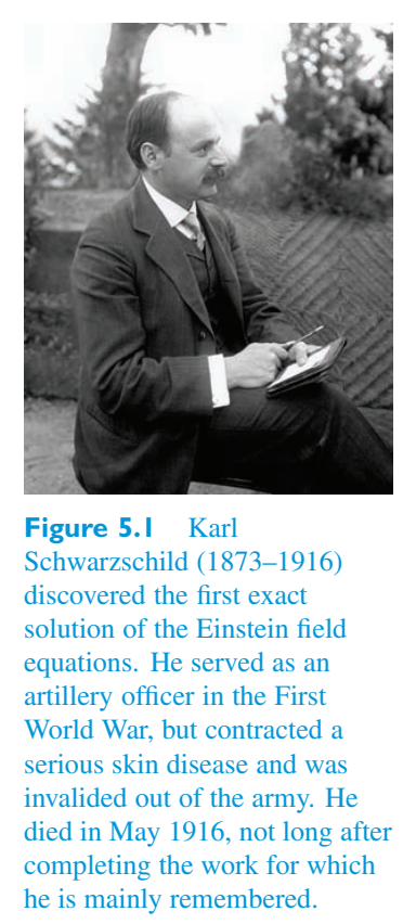
5.1.1 The Schwarzschild metric5.1.1 史瓦西度规
The ‘exterior’ Schwarzschild solution discussed here describes the spacetime geometry in the empty region surrounding a non-rotating, spherically symmetric body of mass M. (You might like to think of that body as a simplified model of a star.) The presentation of the Schwarzschild solution, like that of any solution of the Einstein field equations, involves specifying, as explicit functions of the spacetime coordinates \(x^0\), \(x^1\), \(x_{2}\), \(x^{3}\), the sixteen components of the metric tensor \(g_{\mu\nu}\) that correspond to the energy–momentum tensor \(T_{\mu\nu}\) in the region of interest. In the case of the Schwarzschild solution, the relevant energy–momentum tensor is \(T_{\mu\nu}\) = 0 since we are dealing with the empty region outside the mass distribution. Nonetheless, the symmetry of the region involved suggests that it would be wise to use a system of spherical coordinates originating at the centre of the massive body, and it also seems likely that the solution will involve the mass M in some way. We shall have more to say about the significance of M and the precise meaning of the coordinates later; for the moment we shall simply refer to the coordinates as Schwarzschild coordinates and denote them by \(x^0\) = ct, \(x^1\) = r, \(x_{2}\) = \(\theta\), \(x^{3}\) = \(\phi\).这里讨论的“外部”史瓦西解描述了围绕非旋转、球对称质量体 M 的空白区域中的时空几何。(您可能希望将该物体视为恒星的简化模型。)与爱因斯坦场方程的任何解一样,史瓦西解的表示涉及将对应于能量-动量的度规张量 \(g_{\mu\nu}\) 的十六个分量指定为时空坐标 \(x^0\)、\(x^1\)、\(x_{2}\)、\(x^{3}\) 的显式函数感兴趣区域中的张量 \(T_{\mu\nu}\)。在史瓦西解的情况下,相关的能量-动量张量为 \(T_{\mu\nu}\) = 0,因为我们正在处理质量分布之外的空区域。尽管如此,所涉及区域的对称性表明,使用源自大质量物体中心的球坐标系是明智的,而且解决方案似乎也可能以某种方式涉及质量 M。M的意义以及坐标的具体含义我们稍后再讲;目前,我们将简单地将坐标称为史瓦西坐标,并将其表示为 \(x^0\) = ct、\(x^1\) = r、\(x_{2}\) = \(\theta\)、\(x^{3}\) = \(\phi\)。
Due to the symmetry of the metric tensor, only ten of its sixteen components \(g_{\mu\nu}\) are independent. Moreover, in the particular case of the Schwarzschild solution, thanks to the spherical symmetry, the lack of time-dependence and the judicious choice of coordinates, only four of the components turn out to be non-zero, and none of them depends on \(x^0\). In fact, the solution can be represented by the diagonal matrix由于度规张量的对称性,其十六个分量 \(g_{\mu\nu}\) 中只有十个是独立的。此外,在史瓦西解的特殊情况下,由于球对称性、时间依赖性的缺乏以及坐标的明智选择,只有四个分量结果是非零的,并且它们都不依赖于 \(x^0\)。事实上,该解可以用对角矩阵表示
Though clear, this is a rather cumbersome way of presenting the metric, so it is actually more common to see the non-zero components presented as the metric coefficients in the four-dimensional line element of the spacetime region being described. This is usually written as follows.虽然很清楚,但这是一种相当麻烦的表示度规的方式,因此实际上更常见的是在所描述的时空区域的四维线元素中将非零分量表示为度规系数。通常写成如下。
The Schwarzschild metric史瓦西度规
Although the terminology that we have been using leads us to refer to this expression as a line element, what it really tells us is the functional form of the non-zero components of the metric tensor. Because of this it is often referred to as the Schwarzschild metric. You should also be aware that built into it is the choice that we made regarding the use of an \(x^0\) coordinate to represent time (some authors prefer \(x^{4}\)) and some other decisions regarding signs and symbols. The upshot of all this is that although we have adopted a range of common conventions, you should not be surprised to find that other authors may make different decisions and will therefore write the Schwarzschild solution in a related but different form.尽管我们一直使用的术语使我们将此表达式称为线元素,但它真正告诉我们的是度规张量的非零分量的函数形式。因此,它通常被称为史瓦西度规。您还应该意识到,它内置了我们关于使用 \(x^0\) 坐标来表示时间(一些作者更喜欢 \(x^{4}\))以及有关符号和符号的其他一些决定的选择。所有这一切的结果是,尽管我们采用了一系列通用约定,但您不应惊讶地发现其他作者可能会做出不同的决定,并因此以相关但不同的形式编写史瓦西解决方案。
5.1.2 Derivation of the Schwarzschild metric5.1.2 史瓦西度规的推导
In empty space \(T_{\mu\nu}\) = 0, so the Einstein field equations become在真空中 \(T_{\mu\nu}\) = 0,因此爱因斯坦场方程变为
These equations are known as the vacuum field equations. Multiplying them by \(g_{\mu\nu}\) and contracting over the indices \(\mu\) and \(\nu\) gives这些方程称为真空场方程。将它们乘以 \(g_{\mu\nu}\),然后对指数 \(\mu\) 和 \(\nu\) 进行收缩,得出
that is,那是,
Summing R \(\nu\) \(\nu\) over all values of \(\nu\) gives the curvature scalar R, while summing + δ 3 = 4. Substituting δ \(\nu\) over all possible values of \(\nu\) gives δ 0 + δ 1 + δ 2 these results into Equation 5.5, we get将 R \(\nu\) \(\nu\) 与 \(\nu\) 的所有值相加,得到曲率标量 R,同时求和 + δ 3 = 4。将 δ \(\nu\) 代入 \(\nu\) 的所有可能值,得到 δ 0 + δ 1 + δ 2,这些结果代入公式 5.5,我们得到
showing that \(R=0\) in this case and hence (from the vacuum field equations) that R \(\mu\)\(\nu\) = 0 for all values of \(\mu\) and \(\nu\). Thus the Ricci tensor and the curvature scalar must both vanish for a vacuum solution, but remember, this is not sufficient to make spacetime flat.显示在这种情况下为 \(R=0\),因此(根据真空场方程)对于 \(\mu\) 和 \(\nu\) 的所有值,R \(\mu\)\(\nu\) = 0。因此,对于真空解,里奇张量和曲率标量必须都消失,但请记住,这不足以使时空平坦。
It would be straightforward (though time-consuming) to show that the Schwarzschild metric written down earlier does indeed lead to a vanishing Ricci tensor and therefore is a solution of the vacuum field equations. However, that is not the aim of this section. Rather, our approach here is to write down the most general metric that exhibits the symmetries expected of the Schwarzschild solution and then use the additional requirement that the metric satisfies the vacuum field equations to lead us to a specific metric that will turn out to be the Schwarzschild solution. This is closer to the approach actually followed by Schwarzschild.很容易(尽管很耗时)证明之前写下的史瓦西度规确实会导致里奇张量消失,因此是真空场方程的解。然而,这不是本节的目的。相反,我们这里的方法是写下最通用的度规,该度规表现出史瓦西解所期望的对称性,然后使用该度规满足真空场方程的附加要求来引导我们得到一个特定的度规,该度规将成为史瓦西解。这更接近史瓦西实际上遵循的方法。
Note that you are not expected to remember all the steps in this derivation, but you should be able to follow them and they should provide helpful examples of many of the tensor quantities that were introduced earlier. The derivation omits a lot of detailed algebra, simply quoting results in its place. If you really want to get a feel for relativity, you might like to fill in some of the missing steps, but don’t try this if you are short of time!请注意,您不需要记住此推导中的所有步骤,但您应该能够遵循它们,并且它们应该提供之前介绍的许多张量量的有用示例。该推导省略了许多详细的代数,只是简单地引用结果来代替它。如果你真的想感受一下相对论,你可能想填写一些缺失的步骤,但如果你时间不够,就不要尝试这个!
Since the Schwarzschild solution describes the geometry of the empty spacetime region surrounding a spherically symmetric body, it is natural to use a system of spherical coordinates centred on the middle of that spherically symmetric body (see Figure 5.2). In addition we shall assume the following.由于史瓦西解描述了围绕球对称体的空时空区域的几何形状,因此很自然地使用以球对称体中间为中心的球坐标系(见图 5.2)。此外,我们将假设以下内容。
1. The spacetime far from the spherically symmetric body is flat. This is1、远离球对称体的时空是平坦的。这是
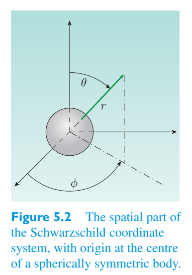
described by saying that the metric is asymptotically flat and is consistent with the idea that gravitational effects become weaker as the distance from their source increases.描述为,该度规是渐近平坦的,并且与引力效应随着距源的距离增加而变弱的想法一致。
2. The metric coefficients do not depend on time. This is described by saying2. 度规系数不依赖于时间。这是通过说来描述的
that the metric is stationary and is consistent with the idea that nothing is moving from place to place.该度规是静止的,并且与没有任何东西从一个地方移动到另一个地方的想法是一致的。
3. The line element is unchanged if t is replaced by − t. This is described by3. 如果将 t 替换为 - t,则线元素不变。这是由
saying that the metric is static and is consistent with the idea that nothing is rotating.说度规是静态的,并且与没有任何东西在旋转的想法是一致的。
We shall say more about these assumptions and about the definition and meaning of the Schwarzschild coordinates later. For the moment we shall simply use them.稍后我们将详细讨论这些假设以及史瓦西坐标的定义和含义。目前我们将简单地使用它们。
The most general spacetime line element that meets all of the listed requirements may be written as满足所有列出的要求的最一般的时空线元素可以写为
where A and B are functions of the radial coordinate r alone. You may wonder why we choose to include exponential functions of the form e 2 A and e 2 B rather than simply using functions such as f (r) and g (r). The reason is that the use of exponentials ensures that the signs of the metric components will be preserved in the desired (+, −, −, −) pattern. The absence of terms proportional to d x i d t (where i = 1, 2 or 3) reflects the static property of the spacetime, while the absence of d x i d x j terms reflects the spherical symmetry.其中 A 和 B 是径向坐标 r 的函数。您可能想知道为什么我们选择包含 e 2 A 和 e 2 B 形式的指数函数,而不是简单地使用 f (r) 和 g (r) 等函数。原因是指数的使用确保了度规分量的符号将保留在所需的 (+, −, −, −) 模式中。缺少与 d x i d t (其中 i = 1、2 或 3) 成比例的项反映了时空的静态特性,而缺少 d x i d x j 项反映了球对称性。
Our aim now is to determine the precise form of the functions A (r) and B (r) using the fact that the metric must satisfy the vacuum field equations. The first step in this process is the determination of the connection coefficients that correspond to the metric given in Equation 5.6. This involves applying the general formula我们现在的目标是利用度规必须满足真空场方程这一事实来确定函数 A (r) 和 B (r) 的精确形式。该过程的第一步是确定与公式 5.6 中给出的度规相对应的联络系数。这涉及应用一般公式
to the case where \(g_{00}=e^{2A}\), \(g_{11}=-e^{2B}\), \(g_{22}=-r^2\) and \(g_{33}=-r^2\sin^2\theta\). Because the metric is represented by a diagonal matrix in this case, each contravariant component \(g^{\mu\nu}\) is simply the reciprocal of the corresponding covariant component, so \(g^{00}=e^{-2A}\), \(g^{11}=-e^{-2B}\), \(g^{22}=-1/r^2\) and \(g^{33}=-1/(r^2\sin^2\theta)\). Substituting these values into the expression for \(\Gamma^\sigma{}_{\mu\nu}\) shows that only nine of the forty independent connection coefficients for this metric are non-zero. Using a prime to indicate differentiation with respect to \(r\), so that \(A'=dA(r)/dr\) and \(B'=dB(r)/dr\), these nine independent non-zero connection coefficients can be written as对于这种情形,有 \(g_{00}=e^{2A}\)、\(g_{11}=-e^{2B}\)、\(g_{22}=-r^2\) 和 \(g_{33}=-r^2\sin^2\theta\)。因为此时度规由对角矩阵表示,所以每个逆变分量 \(g^{\mu\nu}\) 都只是相应协变分量的倒数,因此 \(g^{00}=e^{-2A}\)、\(g^{11}=-e^{-2B}\)、\(g^{22}=-1/r^2\),并且 \(g^{33}=-1/(r^2\sin^2\theta)\)。把这些值代入 \(\Gamma^\sigma{}_{\mu\nu}\) 的表达式可知,该度规的四十个独立联络系数中只有九个非零。用撇号表示对 \(r\) 求导,即 \(A'=dA(r)/dr\)、\(B'=dB(r)/dr\),这九个独立的非零联络系数可写为
These non-zero connection coefficients can be used to determine the non-zero components of the Riemann curvature tensor using the general formula这些非零联络系数可用于使用通用公式确定黎曼曲率张量的非零分量
Again, there are many symmetries so not all the non-zero curvature tensor components are independent, though these are the six that are:同样,存在许多对称性,因此并非所有非零曲率张量分量都是独立的,尽管有以下六个:
where the double prime indicates the second derivative with respect to r. Contraction of the Riemann tensor gives the Ricci tensor with components and reveals (after much algebra) that only the four diagonal components of the Ricci tensor are not identically zero:其中双素数表示关于 r 的二阶导数。黎曼张量的收缩给出了带有分量的里奇张量,并揭示了(经过大量代数计算后),只有里奇张量的四个对角分量不全为零:
Now, we already know that for a vacuum solution all four of these components must be equal to zero. Nonetheless, for the sake of completeness, we shall use the expressions that we have obtained to calculate the curvature scalar现在,我们已经知道对于真空解决方案,所有这四个分量必须等于零。尽管如此,为了完整起见,我们将使用我们获得的表达式来计算曲率标量
which in this case becomes在这种情况下变成
and yields和产量
When evaluated, this too must vanish for a vacuum solution.在评估时,对于真空解决方案来说,这也必须消失。
Combining the results for the curvature scalar and the components of the Ricci tensor, we can determine the Einstein tensor components given by结合曲率标量的结果和 Ricci 张量的分量,我们可以确定爱因斯坦张量分量:
the only ones that are not identically zero in this case being在这种情况下,唯一不完全相同的零是
Now, the vacuum field equations demand that even these Einstein tensor components should each be zero in the space outside the spherically symmetric body. One consequence of this is that e − 2 A G + e − 2 B G = 0, but this implies that现在,真空场方程要求即使是这些爱因斯坦张量分量在球对称体外部的空间中也应该为零。其结果之一是 e − 2 A G + e − 2 B G = 0,但这意味着
implying that \(A'\) + \(B'\) = 0, which can be integrated to give A (r) + B (r) = C, where C is a constant. This constant can be set to zero without loss of generality, since any other choice can be represented by a rescaling of the r -coordinate, which still has an arbitrary scale at this stage. (This is one of the points that we shall return to later.) Making use of this freedom to set C = 0, we see that A (r) = − B (r), and the equation G = 0 can be rewritten as意味着 \(A'\) + \(B'\) = 0,可以积分得到 A (r) + B (r) = C,其中 C 是常数。该常数可以设置为零而不失一般性,因为任何其他选择都可以通过 r 坐标的重新缩放来表示,该坐标在此阶段仍然具有任意比例。(这是我们稍后将讨论的要点之一。)利用这种自由度来设置 C = 0,我们看到 A (r) = − B (r),并且方程 G = 0 可以重写为
e − 2 B = 1 − R/r, which, after ignoring 1/\(r^2\), can also be integrated, to yield where the integration constant, \(R_S\), has the units of distance. The constant \(R_S\) is called the Schwarzschild radius.e − 2 B = 1 − R/r,在忽略 1/\(r^2\) 后,也可以对其进行积分,得到积分常数 \(R_S\) 的单位为距离。常数 \(R_S\) 称为史瓦西半径。
Since e 2 A = e − 2 B, we can now identify the explicit form that must be taken by the two exponential functions in the line element of Equation 5.6 if the corresponding metric is to satisfy the vacuum field equations. Explicitly,由于 e 2 A = e − 2 B,如果相应的度规要满足真空场方程,我们现在可以确定方程 5.6 的线元中的两个指数函数必须采用的显式形式。明确地说,
This shows that the line element of the Schwarzschild solution can be written as这表明史瓦西解的线元可以写为
The final step in our modern derivation is to use the principle of consistency and the Newtonian limit to relate the Schwarzschild radius to the mass \(M\) of the spherically symmetric body centred on the origin. We saw in Section 4.3.3 that, for weak fields in the Newtonian limit, \(g_{00}=1+h_{00}=1+2\Phi/c^2\), where \(\Phi\) is the Newtonian gravitational potential (i.e. the potential energy per unit mass). In the case of a spherically symmetric body of mass \(M\) centred on the origin, the Newtonian gravitational potential outside the body, at a distance \(r\) from the origin, is \(\Phi=-GM/r\). It follows that in the Newtonian limit \(g_{00}=1-2GM/(rc^2)\). Comparing this with the metric coefficient that occupies the position of \(g_{00}\) in Equation 5.7, we see that the two will agree provided that we assign the Schwarzschild radius the value现代推导的最后一步,是利用一致性原理和牛顿极限,把史瓦西半径同以原点为中心的球对称天体质量 \(M\) 联系起来。我们在第 4.3.3 节已经看到,在弱场的牛顿极限下,\(g_{00}=1+h_{00}=1+2\Phi/c^2\),其中 \(\Phi\) 是牛顿引力势(即单位质量的势能)。对于以原点为中心、质量为 \(M\) 的球对称天体,在距原点 \(r\) 处,天体外部的牛顿引力势为 \(\Phi=-GM/r\)。因此,在牛顿极限下 \(g_{00}=1-2GM/(rc^2)\)。将其与方程 5.7 中位于 \(g_{00}\) 位置的度规系数比较可知,只要把史瓦西半径取为下列数值,两者就会一致
We can now represent the metric tensor of the Schwarzschild solution in the diagonal matrix form我们现在可以用对角矩阵形式表示史瓦西解的度规张量
or in its more common form as the line element或者以更常见的形式作为线元素
d s to incremental which relates incremental changes in the spacetime interval changes in intervals of Schwarzschild coordinate time t and the Schwarzschild spatial coordinates r, \(\theta\), \(\phi\) between neighbouring events.d s 为增量,它涉及相邻事件之间史瓦西坐标时间 t 的间隔和史瓦西空间坐标 r、\(\theta\)、\(\phi\) 的时空间隔变化的增量变化。
There are shortcuts that could have been taken in this section; for instance, we could have used the condition that the components of the Ricci tensor must vanish in the case of a vacuum solution rather than working out the Einstein tensor components and applying the full field equations. The approach we have taken has the advantage of showing you explicit examples of each of the major tensor quantities. Now that we know what they look like, we can investigate their meaning and significance in this particular case.在本节中可以采取一些捷径;例如,我们可以使用在真空解的情况下里奇张量的分量必须消失的条件,而不是计算爱因斯坦张量分量并应用全场方程。我们采取的方法的优点是向您展示每个主要张量的明确示例。现在我们知道它们是什么样子了,我们可以研究它们在这个特定案例中的含义和意义。
Exercise 5.1 Confirm the value for \(G_{00}\) given above.练习 5.1 确认上面给出的 \(G_{00}\) 的值。
5.2 Properties of Schwarzschild spacetime5.2 史瓦西时空的性质
Several properties of the Schwarzschild metric were mentioned early in the previous section, where they were used to determine the general line element given in Equation 5.6. One of the most basic was spherical symmetry. We shall start by considering that property in more detail.史瓦西度规的几个属性在上一节的前面已经提到过,它们被用来确定公式 5.6 中给出的一般线元素。最基本的之一是球对称。我们将首先更详细地考虑该属性。
5.2.1 Spherical symmetry5.2.1 球对称性
At any particular value of t, call it T, fixing the value of r to have some particular value R ensures that d t = 0 and d r = 0, and reduces the Schwarzschild line element to在 t 的任何特定值处,将其称为 T,将 r 的值固定为某个特定值 R,确保 d t = 0 且 d r = 0,并将史瓦西线元素减少为
which describes the two-dimensional geometry on the surface of a sphere of radius R. Now, from a physical point of view, no point on this spherical surface is any more ‘special’ than any other point. The fact that no value of \(\phi\) is picked out is clear from the fact that \(\phi\) does not appear in any of the metric coefficients. However, the same is not true of \(\theta\) — that does appear in the metric coefficient that multiplies (d \(\phi\)) 2. This makes it seem that there might be something special about certain values of \(\theta\) even though we have already said that there can’t be. The reason why \(\theta\) is picked out in this way has nothing to do with the gravitation of a spherically symmetric body; it is entirely due to the way in which we define spherical coordinates. When we use such coordinates we have to choose some radial direction to be the ‘north polar axis’. That direction is assigned the special coordinate value \(\theta\) = 0 even though in the case of a non-rotating spherically symmetric body there is nothing physically ‘special’ about the direction chosen to play that role. Any other direction from the origin could just as easily have been chosen as the north polar axis.它描述了半径为 R 的球体表面上的二维几何形状。现在,从物理角度来看,这个球面上的任何点都比任何其他点更“特殊”。从 \(\phi\) 没有出现在任何度规系数中的事实可以清楚地看出,没有选取出 \(\phi\) 的值。然而,\(\theta\) 的情况却并非如此——它确实出现在乘以 (d \(\phi\)) 2 的度规系数中。这使得 \(\theta\) 的某些值看起来可能有一些特殊之处,尽管我们已经说过不可能有。之所以这样选出\(\theta\),与球对称体的万有引力无关;这完全是由于我们定义球坐标的方式造成的。当我们使用这样的坐标时,我们必须选择某个径向方向作为“北极轴”。该方向被分配特殊坐标值 \(\theta\) = 0,即使在非旋转球对称体的情况下,选择扮演该角色的方向在物理上没有什么“特殊”之处。从原点开始的任何其他方向都可以很容易地选择为北极轴。
This illustrates an important point in general relativity that we shall come back to later. Locations that appear to be ‘special’ in metrics and line elements may be physically special in some way, or they may only appear to be special because of some particular feature of the coordinate system being used. It is always important to distinguish between real physical effects and non-physical effects produced by the coordinate system alone. The need for this distinction is clear, but as you will soon see it is not always easy to tell whether a particular feature is the result of coordinates or gravitation.这说明了广义相对论中的一个重要观点,我们稍后会再讨论。在度规和线元素中看起来“特殊”的位置可能在某种程度上在物理上是特殊的,或者它们可能只是因为所使用的坐标系的某些特定特征而显得特殊。区分真实的物理效应和仅由坐标系产生的非物理效应始终很重要。这种区分的必要性是显而易见的,但正如您很快就会看到的那样,辨别某个特定特征是坐标还是引力的结果并不总是那么容易。
The Schwarzschild solution is spherically symmetric: at any given value of t, all points with the same value of r are physically equivalent. The spacetime has the same symmetries as a sphere (by which mathematicians mean it has the symmetries of the surface of a ball), so it is said to be ‘invariant under rotations about the origin’ (see Figure 5.3).史瓦西解是球对称的:在任何给定的 t 值下,所有具有相同 r 值的点在物理上是等效的。时空与球体具有相同的对称性(数学家认为它具有球表面的对称性),因此被称为“绕原点旋转不变”(见图 5.3)。
Of course, this does not mean that points with different values of r are physically equivalent. Indeed, we have already seen that in the Newtonian limit, points at different values of r will correspond to different values of the gravitational potential. Also, one of the main outcomes of the derivation was that the metric coefficients in the Schwarzschild line element contain terms of the form 1 − 2 GM/\(c^2\) r that are functions of r.当然,这并不意味着r值不同的点在物理上是等价的。事实上,我们已经看到,在牛顿极限下,不同 r 值的点将对应不同的引力势值。此外,推导的主要结果之一是史瓦西线元素中的度规系数包含 1 − 2 GM/\(c^2\) r 形式的项,它们是 r 的函数。
system ct, r, \(\theta\), \(\phi\)系统 ct、r、\(\theta\)、\(\phi\)
Exercise 5.2 Suppose that the Schwarzschild coordinate练习 5.2 假设史瓦西坐标
used to describe the spacetime outside a non-rotating spherically symmetric body ct, r, \(\theta\), \(\phi'\), where is replaced by a different system that uses the coordinates \(\phi'\) = \(\phi\) + \(\phi\).用于描述非旋转球对称体 ct, r, \(\theta\), \(\phi'\) 外部的时空,其中被使用坐标 \(\phi'\) = \(\phi\) + \(\phi\) 的不同系统替换。
(a) Show that the Schwarzschild metric is form-invariant when the new coordinates are substituted for the old ones.(a) 证明当新坐标替换旧坐标时,史瓦西度规是形式不变的。
(b) Give a physical justification for the mathematical fact stated in part (a).(b) 对 (a) 部分所述的数学事实给出物理论证。
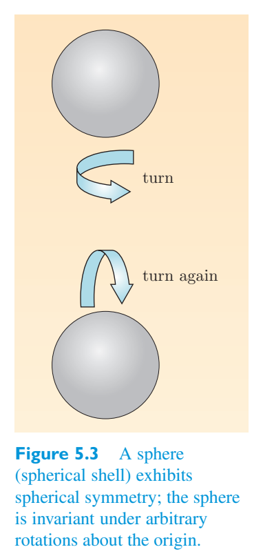
5.2.2 Asymptotic flatness5.2.2 渐近平坦度
In the Schwarzschild line element, the factor 1 − 2 GM/\(c^2\) r appears in the metric coefficients of the \(c^2\) (d t) 2 term and the (d r) 2 term. The factor is independent of direction and approaches 1 as r becomes large. The meaning of ‘large’ in this context depends on the value of M; what is meant is that r is sufficiently large to make the term 2 GM/\(c^2\) r very much smaller than 1. Where that condition is satisfied, 1 − 2 GM/\(c^2\) r → 1 and the Schwarzschild line element在史瓦西线元中,因子 1 − 2 GM/\(c^2\) r 出现在 \(c^2\) (d t) 2 项和 (d r) 2 项的度规系数中。该因子与方向无关,并且随着 r 变大而接近 1。在这种情况下,“大”的含义取决于 M 的值;这意味着 r 足够大,使得 2 GM/\(c^2\) r 项远小于 1。如果满足该条件,则 1 − 2 GM/\(c^2\) r → 1 和史瓦西线元
takes the form of the Minkowski line element采用闵可夫斯基线元的形式
that describes the flat spacetime of special relativity in spherical coordinates. This is the form that we should expect the Schwarzschild line element to take ‘far’ from the origin where gravitational effects due to the mass of the spherically symmetric body will be negligible.它描述了球坐标中狭义相对论的平坦时空。这是我们应该期望史瓦西线元远离原点的形式,其中球对称体质量引起的引力效应可以忽略不计。
Remembering that this ‘flatness’ only applies at sufficiently large values of r, we say that the Schwarzschild metric has the property of asymptotic flatness.请记住,这种“平坦度”仅适用于足够大的 r 值,我们说史瓦西度规具有渐近平坦度的属性。
5.2.3 Time-independence5.2.3 时间无关性
Two other properties of the Schwarzschild metric that were briefly mentioned earlier related to its time-independence. The first of these is the property of being stationary, implying that none of the metric coefficients depends on t. So, if t 1 and \(t_{2}\) represent the time coordinates of neighbouring events, then d t = t − t = (t + t) − (t + t) = \(t'\) − \(t'\) = d \(t'\), and the metric is invariant under a coordinate transformation of the form t → \(t'\) = t + \(t_0\), where \(t_0\) is a constant. This specific aspect of time-independence is described as ‘invariance under translation in time’ and is another symmetry of the solution.前面简要提到的史瓦西度规的另外两个属性与其时间无关性有关。第一个是平稳的属性,这意味着没有一个度规系数依赖于 t。因此,如果 t 1 和 \(t_{2}\) 表示相邻事件的时间坐标,则 d t = t − t = (t + t) − (t + t) = \(t'\) − \(t'\) = d \(t'\),并且在 t → \(t'\) = t + \(t_0\) 形式的坐标变换下,度规是不变的,其中 \(t_0\) 是常数。时间无关的这一特定方面被描述为“时间平移下的不变性”,并且是该解决方案的另一种对称性。
The second feature relating to time-independence introduced earlier was the property of being static. This concerns invariance under transformations that reverse time, such as t → − t. The fact that the Schwarzschild metric is stationary ensures that time reversal will have no effect on any of the metric coefficients since they do not depend on t at all. However, in order that the metric should be static, it is also important that the line element should not contain any terms of the form d r d t, d \(\theta\) d t or d \(\phi\) d t. Such terms are often referred to as ‘cross terms’ or ‘mixed terms’ and are typical of situations involving rotation.前面介绍的与时间无关的第二个特征是静态属性。这涉及到逆转时间的变换下的不变性,例如 t → − t。史瓦西度规是平稳的事实确保时间反转不会对任何度规系数产生影响,因为它们根本不依赖于 t。然而,为了使度规应该是静态的,线元素不应包含任何形式为 d r d t、d \(\theta\) d t 或 d \(\phi\) d t 的项也很重要。此类术语通常称为“交叉术语”或“混合术语”,是涉及轮换的典型情况。
The Schwarzschild metric is both stationary and static.史瓦西度规既是平稳的又是静态的。
5.2.4 Singularity5.2.4 奇点
A striking feature of the Schwarzschild metric is its odd behaviour as \(r\) approaches the Schwarzschild radius \(R_S=2GM/c^2\). As \(r\to R_S\), the factor \(1-R_S/r\) causes the metric coefficient \(g_{00}\) to approach zero, while the factor \((1-R_S/r)^{-1}\) causes \(g_{11}\) to diverge. The unlimited growth of the latter factor is described by saying that there is a singularity in the Schwarzschild metric. This particular singularity is in fact a consequence of the coordinates that we are using to describe the Schwarzschild solution. That is, it is a coordinate singularity, not a physically meaningful gravitational singularity. As a coordinate singularity it can be removed by an appropriate transformation of coordinates in a way that would not be possible for a true gravitational singularity. Nonetheless it is a feature of the solution as described by Schwarzschild coordinates and an indicator of the significance of \(R_S\).史瓦西度规的一个显著特征,是当 \(r\) 接近史瓦西半径 \(R_S=2GM/c^2\) 时会出现特殊行为。当 \(r\to R_S\) 时,因子 \(1-R_S/r\) 使度规系数 \(g_{00}\) 趋于零,而因子 \((1-R_S/r)^{-1}\) 使 \(g_{11}\) 发散。后一因子的无界增长通常表述为史瓦西度规中存在一个奇点。这个特殊奇点实际上来自我们用来描述史瓦西解的坐标;也就是说,它是坐标奇点,而不是具有物理意义的引力奇点。作为坐标奇点,它可以通过适当的坐标变换消除,而真正的引力奇点不可能这样消除。尽管如此,它仍然是用史瓦西坐标描述该解时的一个特征,也标志着 \(R_S\) 的重要性。
When considering this coordinate singularity it is important to remember that the exterior Schwarzschild solution that we are discussing describes the spacetime outside a spherically symmetric body of mass M. It is therefore interesting to ask if \(R_S\) is likely to be larger or smaller than the radius of such a body. If \(R_S\) is smaller than the body’s radius, the coordinate singularity will be outside the domain in which the Schwarzschild solution is applicable, and the solution itself will be non-singular throughout the region that it actually describes.在考虑这个坐标奇点时,重要的是要记住,我们正在讨论的史瓦西外解描述了质量为 M 的球对称体外部的时空。因此,询问 \(R_S\) 是否可能大于或小于这样一个物体的半径是很有趣的。如果 \(R_S\) 小于物体的半径,则坐标奇点将位于史瓦西解适用的域之外,并且解本身在其实际描述的整个区域中将是非奇异的。
For a body with the mass of the Sun (about \(2.0\times10^{30}\) kg), the Schwarzschild radius is 3.0 km. This compares with a solar radius of about 0.7 million km. So in the case of a normal star-like body, the Schwarzschild radius is deep inside the body. Of course, not all bodies of astronomical interest are ‘normal’ or ‘star-like’. As you will see later, the Schwarzschild radius is of great importance in the study of black holes. A body can become a black hole if its surface shrinks within its Schwarzschild radius.对于质量相当于太阳(大约 \(2.0\times10^{30}\) kg)的天体,史瓦西半径为 3.0 公里。相比之下,太阳半径约为 70 万公里。因此,对于正常的类星体来说,史瓦西半径位于物体内部深处。当然,并非所有具有天文意义的天体都是“正常”或“类星体”。正如您稍后将看到的,史瓦西半径在黑洞研究中非常重要。如果一个物体的表面收缩到史瓦西半径内,它就会变成黑洞。
A final point to note is that the Schwarzschild metric also has a singularity at r = 0. This is a gravitational singularity, marked by the unlimited growth of invariants related to the curvature, and cannot be removed by any change of coordinates. This singularity is of little relevance to the exterior solution that we have been discussing in this section, but it will be significant when we come to discuss black holes.最后要注意的一点是,史瓦西度规在 r = 0 处也有一个奇点。这是一个引力奇点,其特征是与曲率相关的不变量无限增长,并且不能通过任何坐标变化来消除。这个奇点与我们在本节中讨论的外部解决方案关系不大,但当我们讨论黑洞时它将很重要。
5.2.5 Generality5.2.5 通用性
According to the Schwarzschild solution, the spacetime geometry outside a static spherically symmetric body is characterized by a single quantity M, which represents the total mass of that distribution.根据史瓦西解,静态球对称体外部的时空几何结构由单个量 M 来表征,它代表该分布的总质量。
In 1923 the American mathematician George Birkhoff proved that even if the source of gravitation is not static (and therefore not necessarily stationary), and as long as its effect is isotropic (i.e. the same in all directions), the vacuum solution of the Einstein field equations in the region exterior to the source is still stationary and is still the Schwarzschild solution.1923年,美国数学家乔治·伯克霍夫证明,即使引力源不是静态的(因此不一定是静止的),只要其效应是各向同性的(即在所有方向上都相同),引力源外部区域的爱因斯坦场方程的真空解仍然是静止的,并且仍然是史瓦西解。
This result is known as Birkhoff’s theorem. One of its implications is that a spherically symmetric body that is expanding or contracting in a purely radial way, or even one that is pulsating radially, cannot produce any gravitational signs of that radial motion beyond the spherical region that contains the material of the body itself. So, if a fixed mass M were contained within a sphere of radius r 1, then the Schwarzschild metric would apply throughout the region r > r 1, but if the mass distribution were to shrink in an isotropic way to a smaller radius \(r^2\), then the spacetime would be unaffected in the region r > r 1 but now region r > \(r^2\). the Schwarzschild metric would apply throughout the larger这个结果被称为伯克霍夫定理。它的含义之一是,以纯径向方式膨胀或收缩的球对称物体,甚至是径向脉动的球对称物体,都不能在包含物体本身材料的球形区域之外产生任何径向运动的引力符号。因此,如果固定质量 M 包含在半径为 r 1 的球体内,则史瓦西度规将适用于整个区域 r > r 1,但如果质量分布以各向同性方式收缩到更小的半径 \(r^2\),则时空在区域 r > r 1 中将不受影响,但现在区域 r > \(r^2\)。史瓦西度规将适用于整个更大的
This is a surprising result. It indicates the special nature of vacuum solutions as well as the generality of the Schwarzschild solution. As you will see later when we discuss gravitational radiation, it also indicates that sources that only pulsate radially cannot produce gravitational waves.这是一个令人惊讶的结果。它表明了真空解的特殊性以及史瓦西解的普遍性。正如您稍后在讨论引力辐射时会看到的那样,它也表明仅径向脉动的源无法产生引力波。
To summarize, we have the following.总而言之,我们有以下几点。
Properties of the Schwarzschild solution史瓦西溶液的性质
The Schwarzschild metric is a static (and therefore stationary), spherically symmetric solution of the Einstein field equations in the empty region exterior to any distribution of energy and momentum characterized by mass M that produces purely isotropic effects in that region. The solution is asymptotically flat, approaching the Minkowski metric in spherical coordinates for sufficiently large values of r. The solution has a coordinate GM/\(c^2\) and a singularity at the Schwarzschild radius r = \(R_S\) = 2 gravitational singularity at r = 0, though neither of these singularities is within the region described by the solution for normal ‘star-like’ bodies.史瓦西度规是爱因斯坦场方程的静态(因此是静止的)球对称解,位于以质量 M 为特征的任何能量和动量分布外部的空区域中,在该区域中产生纯各向同性效应。对于足够大的 r 值,该解是渐近平坦的,接近球坐标中的闵可夫斯基度规。该解具有坐标 GM/\(c^2\) 和史瓦西半径 r = \(R_S\) = 2 处的奇点(r = 0),尽管这些奇点都不在正常“星状”天体的解所描述的区域内。
5.3 Coordinates and measurements in Schwarzschild spacetime5.3 史瓦西时空中的坐标和测量
We now need to deal with an issue that has been present since we first introduced the Schwarzschild coordinates ct, r, \(\theta\), \(\phi\) near the start of this chapter. The issue concerns the relationship between coordinate values and physically meaningful intervals of time and distance.我们现在需要处理一个自从我们在本章开头首次介绍史瓦西坐标 ct, r, \(\theta\), \(\phi\) 以来就一直存在的问题。该问题涉及坐标值与物理上有意义的时间和距离间隔之间的关系。
When confronted by a system of coordinates that includes a t -coordinate and an r -coordinate, it is tempting to assume that the t must represent time and the r radial distance from the origin. However, such an assumption is always dangerous and often wrong.当面对包含 t 坐标和 r 坐标的坐标系时,人们很容易认为 t 必须代表时间,r 代表距原点的径向距离。然而,这样的假设总是危险的,而且常常是错误的。
The simple fact is that in general relativity, coordinates are essentially arbitrary systems of markers chosen to distinguish one event from another. This gives us great freedom in how we define coordinates, a freedom that we exploited in the derivation of the Schwarzschild metric. The relationship between the coordinate differences separating events and the corresponding intervals of time or distance that would be measured by a specified observer must be worked out using the metric of the spacetime. It cannot be assumed that the ‘physical’ times and distances that would be measured by clocks or measuring sticks are directly specified by the coordinates. This situation is described by saying that:简单的事实是,在广义相对论中,坐标本质上是为区分一个事件与另一个事件而选择的任意标记系统。这为我们定义坐标提供了很大的自由度,我们在推导史瓦西度规时也利用了这种自由度。分隔事件的坐标差与指定观察者测量的相应时间或距离间隔之间的关系必须使用时空度规来计算。不能假设时钟或量尺测量的“物理”时间和距离是直接由坐标指定的。这种情况是这样描述的:
In general relativity, coordinates do not have immediate metrical significance.在广义相对论中,坐标不具有直接的度规意义。
Einstein found this a perplexing feature of general relativity. In his own account of how the general theory developed after 1908 he says:爱因斯坦发现这是广义相对论的一个令人困惑的特征。在他自己关于 1908 年之后一般理论如何发展的描述中,他说:
Why were another seven years required for the construction of the general theory of relativity? The main reason lies in the fact that it is not easy to free oneself from the idea that coordinates must have an immediate metrical meaning.为什么广义相对论的构建又需要七年时间?主要原因在于,要摆脱“坐标必须具有直接的度规意义”这一观念并不容易。
Quoted in Schilpp, P. A. (ed.) (1969) Albert Einstein — Philosopher Scientist, 3rd edn, Illinois, Open Court.引自 Schilpp, P. A. (ed.) (1969) Albert Einstein — Philosopher Scientist,第 3 版,伊利诺伊州,公开法庭。
Intervals of time and distance must be measured by an observer who must make use of a frame of reference, so we start with a discussion of the observers and frames that will be relevant to our discussion of Schwarzschild spacetime.时间和距离的间隔必须由必须使用参考系的观察者来测量,因此我们首先讨论与我们对史瓦西时空的讨论相关的观察者和参考系。
5.3.1 Frames and observers5.3.1 框架和观察者
We saw in the discussion of special relativity that the phenomena of time dilation and length contraction made it important to be clear about who was performing measurements of time and distance, and to be especially careful when relating time and distance measurements made by different inertial observers. In special relativity, inertial fames are ‘global’, in principle stretching out to infinity. We needed to be clear about the frame that an observer was using but we emphasized the distinction between ‘seeing’ and ‘observing’, and stressed that observers were concerned with the latter, which made their location irrelevant for most purposes.我们在狭义相对论的讨论中看到,时间膨胀和长度收缩的现象使得弄清楚谁在进行时间和距离测量非常重要,并且在关联不同惯性观察者进行的时间和距离测量时要特别小心。在狭义相对论中,惯性名声是“全球性的”,原则上可以延伸到无穷大。我们需要清楚观察者使用的框架,但我们强调“看到”和“观察”之间的区别,并强调观察者关心的是后者,这使得他们的位置与大多数目的无关。
In general relativity, the situation is very different. There is no ‘special’ class of frames, and the frames that are used are generally ‘local’ so an observer’s location is important. In this chapter we shall be particularly concerned with observations made in three ‘local’ frames: the frame used by a freely falling observer, a frame that is at rest at some specified location, and the frame of a ‘distant’ observer located far from the spherically symmetric body at the origin of Schwarzschild coordinates. The frame of the freely falling observer is locally inertial; gravity has effectively been ‘turned off’ and special relativity applies locally. The observer at a fixed location will need to take steps to avoid falling freely; they might need to locate themselves in a rocket, for example. For such an observer special relativity will work locally but only if the observer supposes that every body is subject to a ‘gravitational force’ that is proportional to the mass of the body. This is really a ‘fictitious force’, introduced to account for the fact that the observer’s frame is not freely falling and is therefore not really locally inertial. To this extent the observer maintaining a fixed position is in a similar situation to a passenger in a bus turning a corner who ‘feels’ the effect of a (fictitious) centrifugal force. The distant observer will be in a region of spacetime that is effectively flat, so special relativity will again apply locally and there will not be any local effects of gravitation to take into account. Such an observer can remain at rest without needing the support of a rocket and can even be regarded as falling freely while remaining at rest!在广义相对论中,情况就大不相同了。没有“特殊”类别的框架,并且使用的框架通常是“本地”的,因此观察者的位置很重要。在本章中,我们将特别关注在三个“局部”坐标系中进行的观察:自由落体观察者使用的坐标系、在某个特定位置静止的坐标系以及位于史瓦西坐标原点远离球对称体的“远距离”观察者的坐标系。自由落体观察者的坐标系具有局部惯性;引力实际上已被“关闭”,狭义相对论在局部适用。固定位置的观察者需要采取措施避免自由落体;例如,他们可能需要在火箭中定位自己。对于这样的观察者来说,狭义相对论将在局部起作用,但前提是观察者假设每个物体都受到与物体质量成正比的“引力”。这实际上是一种“虚拟力”,引入它是为了解释观察者的框架不是自由落体的,因此并不是真正的局部惯性。从这个意义上说,保持固定位置的观察者与公交车上转弯的乘客处于类似的情况,“感觉到”(虚构的)离心力的作用。遥远的观察者将处于一个实际上平坦的时空区域,因此狭义相对论将再次适用于局部,并且不会考虑任何引力的局部效应。这样的观察者不需要火箭的支撑就可以保持静止,甚至可以视为静止状态下自由落体!
5.3.2 Proper time and gravitational time5.3.2 本征时和引力时
dilation扩张
Consider two events involving the emission of light, that happen in the Schwarzschild spacetime surrounding a static spherically symmetric body. Suppose that the two emission events are described by the Schwarzschild coordinates (t, r, \(\theta\), \(\phi\)) and (t + d t, r, \(\theta\), \(\phi\)), so they are separated by a difference in coordinate time \(dt_{\rm em}\), while their other coordinate separations are all zero: d r = d \(\theta\) = d \(\phi\) = 0.考虑两个涉及光发射的事件,这两个事件发生在围绕静态球对称体的史瓦西时空中。假设两个发射事件由史瓦西坐标 (t, r, \(\theta\), \(\phi\)) 和 (t + d t, r, \(\theta\), \(\phi\)) 描述,因此它们之间的坐标时间差为 \(dt_{\rm em}\),而它们的其他坐标间隔均为零: d r = d \(\theta\) = d \(\phi\) = 0。
According to the Schwarzschild metric, the infinitesimal spacetime separation of these events is given by根据史瓦西度规,这些事件的无穷小时空分离由下式给出
and the proper time between the events, as would be measured by a clock at rest at the location of the events, is \(d\tau_{\rm em}\) = d s em/c, so事件之间的固有时间(通过事件所在位置的静止时钟测量)为 \(d\tau_{\rm em}\) = d s em/c,因此
Note that the proper time separating the events, according to a stationary clock at the location of the events, is less than the coordinate time separating the events.注意,根据事件位置处的固定时钟,分隔事件的正确时间小于分隔事件的坐标时间。
Now consider what will be seen by an observer at rest at some other location with the same angular coordinates \(\theta\) and \(\phi\) but a different value of the radial coordinate r = \(r_{\rm ob}\). As will be shown in Chapter 6, such an observer will find that the coordinate time separating the signals from the two events when they arrive at r = \(r_{\rm ob}\) will be the same as the coordinate time between the emission of those signals. We can indicate this by writing \(dt_{\rm ob}\) = \(dt_{\rm em}\). All the other coordinate differences d r, d \(\theta\) and d \(\phi\) will still be zero. It follows that the spacetime separation between the observations of the two signals现在考虑一下在其他位置静止的观察者会看到什么,该位置具有相同的角坐标 \(\theta\) 和 \(\phi\),但径向坐标 r = \(r_{\rm ob}\) 的值不同。正如第 6 章所示,这样的观察者会发现,当信号到达 r = \(r_{\rm ob}\) 时,将信号与两个事件分开的坐标时间将与这些信号发射之间的坐标时间相同。我们可以通过写 \(dt_{\rm ob}\) = \(dt_{\rm em}\) 来表示这一点。所有其他坐标差 d r、d \(\theta\) 和 d \(\phi\) 仍将为零。由此可见,两个信号的观测值之间的时空间隔
and the proper time between the observations of the two signals will be两个信号观测之间的固有时间为
There are two important consequences that follow from these relationships.这些关系产生两个重要的后果。
First, for a distant observer fixed at a sufficiently large value of r, effectively at \(r_{\rm ob}\) = ∞, it follows from Equation 5.14 that首先,对于固定在足够大的 r 值(实际上 \(r_{\rm ob}\) = ∞)的远处观察者,根据公式 5.14 可得出:
Integrating both sides of this equation shows that even for two emission events separated by a finite coordinate time difference \(\Delta t\) em, that difference will still equal \(\Delta \tau\) ∞, the difference in the proper time between observations of those events made by a stationary observer at infinity. This establishes that the Schwarzschild coordinate time separating two events at a fixed location can actually be determined by measuring the proper time between observations of those two events using a stationary clock at infinity. This gives us a way, in principle at least, of assigning Schwarzschild coordinate times to events.对该方程两边进行积分表明,即使对于由有限坐标时间差 \(\Delta t\) em 分隔开的两个发射事件,该差值仍将等于 \(\Delta \tau\) ∞,即无穷远静止观察者对这些事件的观测之间的本征时间差。这表明,在固定位置分隔两个事件的史瓦西坐标时间实际上可以通过使用无穷远处的固定时钟测量这两个事件的观察之间的固有时间来确定。至少在原则上,这为我们提供了一种为事件分配史瓦西坐标时间的方法。
- ● Should we be worried by the fact that this argument involves an observer at我们应该担心这一论点涉及观察员吗?
infinity? Does that invalidate the process?无穷大?这会使该过程无效吗?
❍ No. All it means is that the observer should be far enough away to be in the asymptotically flat region of spacetime where 2 GM/\(c^2\) \(r_{\rm ob}\) is negligible compared with 1.❍ 不。它的意思是观察者应该足够远,处于渐进平坦的时空区域,其中 2 GM/\(c^2\) \(r_{\rm ob}\) 与 1 相比可以忽略不计。
Second, it follows from Equation 5.15 and the relation between \(d\tau_{\rm em}\) and \(dt_{\rm em}\) in Equation 5.12 that其次,根据公式 5.15 以及公式 5.12 中 \(d\tau_{\rm em}\) 和 \(dt_{\rm em}\) 之间的关系可以得出:
This shows that the proper time between the observation of the two light signals at infinity, d \(\tau\) ∞, is greater than the proper time between their emission as measured at the site of the emission, \(d\tau_{\rm em}\).这表明在无穷远处观察两个光信号之间的本征时间 d \(\tau\) ∞ 大于在发射地点测量的它们的发射之间的本征时间 \(d\tau_{\rm em}\)。
If we suppose that the two events that we have been discussing represent the beginning and the end of a single tick of a clock fixed at r = \(r_{\rm em}\), then our second result shows that the duration of that tick as seen by a distant observer will be如果我们假设我们一直在讨论的两个事件代表固定在 r = re em 的时钟的单个滴答声的开始和结束,那么我们的第二个结果表明,远处观察者看到的该滴答声的持续时间将是
increased by a factor 1/1 − 2 GM. This shows that the distant observer will find that the clock at r = \(r_{\rm em}\) is running slow.GM 增加了 1/1 − 2 倍。这表明远处的观察者会发现 r = re em 处的时钟运行缓慢。
- ● If the stationary clock emitting the light signals was moved closer to the如果发射光信号的固定时钟移近
surface of the spherically symmetric body, how would the observations of its rate of ticking by a distant fixed observer be affected?球对称体的表面,远距离固定观察者对其滴答速率的观测会受到怎样的影响?
❍ The distant observer would find that the clock ticked even more slowly. Moving the clock closer to the surface reduces the value of \(r_{\rm em}\), which has the❍ 远处的观察者会发现时钟走得更慢。将时钟移近表面会降低 re em 的值,其中
effect of increasing the factor 1/1 − 2 GM.增加系数 1/1 − 2 GM 的效果。
This effect, the slowing of the rate of ticking of a clock in a gravitational field, as seen by a distant observer, is sometimes referred to as gravitational time dilation. Note, however, that there is a significant difference between this effect and the time dilation in special relativity that we studied in Chapter 1. In that earlier case we were careful to ignore the effects of signal travel time and only considered the time intervals between the events themselves as measured by different inertial observers, irrespective of the observer’s location. In the general relativistic case there is no relative motion; both the clock and the distant observer are at rest, and we are very deliberately considering the proper time between the arrival of light signals at that distant observer’s location. The distant observer is still making observations, but the observations are of local events — the arrival of the light signals, not their emission.这种效应,即引力场中时钟的滴答速度减慢,如远处观察者所见,有时被称为引力时间膨胀。但请注意,这种效应与我们在第一章中研究的狭义相对论中的时间膨胀之间存在显着差异。在之前的例子中,我们小心地忽略了信号传播时间的影响,只考虑了由不同惯性观察者测量的事件本身之间的时间间隔,而不管观察者的位置如何。在广义相对论情况下,不存在相对运动;时钟和远处的观察者都处于静止状态,我们正在非常仔细地考虑光信号到达远处观察者位置之间的固有时间。远处的观察者仍在进行观察,但观察的是局部事件——光信号的到达,而不是它们的发射。
The general relativistic effect can be given another interpretation. Suppose that the two ‘emission’ events represent the emission of successive peaks of an electromagnetic wave (a light wave), so that \(d\tau_{\rm em}\) represents the period of that wave at its point of emission. Then \(d\tau_{\rm ob}\) will represent the period of that same radiation as measured by a distant observer. The periods will still be related by广义相对论效应可以有另一种解释。假设两个“发射”事件代表电磁波(光波)连续峰值的发射,因此 \(d\tau_{\rm em}\) 代表该波在发射点的周期。那么 \(d\tau_{\rm ob}\) 将代表由远处观察者测量的相同辐射的周期。这些期间仍将通过以下方式相关
but now we can say that the reciprocal of the period represents the frequency of the radiation, so the frequency observed by the distant observer will be但现在我们可以说周期的倒数代表辐射的频率,因此远处观察者观测到的频率将是
This shows that the observed (proper) frequency is less than the emitted (proper) frequency. It follows that light rising through a gravitational field will be redshifted. This phenomenon is known as gravitational redshift (see Figure 5.4). You saw in Section 4.1.1 that a local version of this phenomenon was already predicted as a consequence of the principle of equivalence. Now, with the aid of the Einstein field equations and the Schwarzschild metric, you can see the full effect, not limited to a local frame, but relating quantities that might be measured in two widely separated local frames. This is an effect that might be measured by an astronomer, and we shall discuss such measurements in Chapter 7.这表明观察到的(正确的)频率小于发射的(正确的)频率。由此可见,穿过引力场的光将会发生红移。这种现象称为引力红移(见图 5.4)。您在第 4.1.1 节中看到,作为等效原理的结果,已经预测了这种现象的局部版本。现在,借助爱因斯坦场方程和史瓦西度规,您可以看到完整的效果,不仅限于局部框架,而且还可以在两个相距较远的局部框架中测量到相关的量。天文学家可以测量这种效应,我们将在第 7 章中讨论此类测量。
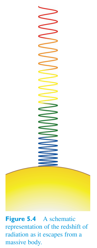
Exercise 5.3 Treating the Sun as a non-rotating, spherically练习 5.3 将太阳视为不旋转的球体
symmetric body, and regarding the surrounding space as well described by the Schwarzschild metric, at what value of the Schwarzschild coordinate r do intervals of proper 1 part in 10 8? time d \(\tau\) and coordinate time d t differ by no more than对称体,并且考虑到由史瓦西度规描述的周围空间,在史瓦西坐标 r 的什么值处,10 8 中的真 1 部分的间隔?时间 d \(\tau\) 与坐标时间 d t 相差不大于
To summarize, we have the following.总而言之,我们有以下几点。
Proper time and gravitational time dilation本征时间和引力时间膨胀
The Schwarzschild coordinate time separating two events at a fixed location is equal to the proper time between sightings of those two events by a distant stationary observer.在固定位置分隔两个事件的史瓦西坐标时间等于远处固定观察者看到这两个事件之间的固有时间。
The rate of ticking of a stationary clock at Schwarzschild coordinate史瓦西坐标下静止时钟的滴答率
distance r will be seen to be slowed by a factor of as measured by a distant stationary observer. This same effect will lead to a gravitational redshift — seen as a reduction in frequency by a factor由远处的静止观察者测量,距离 r 将被减慢 1 倍。同样的效应将导致引力红移——被视为频率降低一个因子
— of the radiation from a stationary source as measured by a distant stationary observer.——由远处的固定观察者测量的固定源的辐射。
5.3.3 Proper distance5.3.3 固有距离
Just as we related differences in Schwarzschild coordinate time to intervals of proper time that might be measured by clocks, so we must relate differences in Schwarzschild coordinate position to proper distances that might be measured using measuring sticks. Consider two events that happen in Schwarzschild spacetime at the same coordinate time but at infinitesimally separated positions, so that their spacetime separation is given by the negative quantity正如我们将史瓦西坐标时间的差异与可以通过时钟测量的固有时间间隔联系起来一样,我们也必须将史瓦西坐标位置的差异与可以使用测量棒测量的固有距离联系起来。考虑在史瓦西时空中发生在同一坐标时间但位置无限小的两个事件,因此它们的时空间隔由负量给出
The proper distance between those two events will be given by d \(\sigma\) = − (d s) 2.这两个事件之间的固有距离由 d \(\sigma\) = − (d s) 2 给出。
We saw earlier, when discussing the spherical symmetry of the Schwarzschild solution (see Subsection 5.2.1), that the events occurring at fixed values of t and r form a spherical shell described by the familiar metric of such a shell. To this extent the Schwarzschild spacetime can be regarded as consisting of a set of nested spheres surrounding the spherically symmetric body. The proper distance between neighbouring points on the sphere of coordinate radius r is given by我们之前在讨论史瓦西解的球对称性时看到(参见第 5.2.1 小节),在 t 和 r 的固定值处发生的事件形成一个球壳,由这种球壳的熟悉度规来描述。从这个意义上说,史瓦西时空可以被视为由一组围绕球对称体的嵌套球体组成。坐标半径为 r 的球体上相邻点之间的固有距离由下式给出
There is nothing unusual about the geometry of any of these spherical surfaces; the sphere of coordinate radius r has proper circumference 2 πr and proper area 4 πr 2. In principle either of these quantities could be measured using ordinary measuring rods. This provides a method, in principle at least, of determining the Schwarzschild radial coordinate r of any event: use measuring sticks to measure the proper circumference C of a circle centred on the origin that passes through the location of the event, then divide that circumference by 2 \(\pi\) to find the coordinate radius r = C/2 \(\pi\).这些球面的几何形状并没有什么异常之处。坐标半径为 r 的球体的固有周长为 2 πr,真面积为 4 πr 2。原则上,这些量中的任何一个都可以使用普通的测量杆来测量。这至少在原则上提供了一种确定任何事件的史瓦西径向坐标 r 的方法:使用测量棒测量以原点为中心、穿过事件位置的圆的固有周长 C,然后将该周长除以 2 \(\pi\) 即可找到坐标半径 r = C/2 \(\pi\)。
What is unusual is that the radial coordinate r does not provide a direct measure of the proper radius of such a sphere, and differences in the radial coordinate r do not indicate the proper distance between different spherical shells. Consider two events that occur at the same coordinate time and with the same angular coordinates \(\theta\) and \(\phi\) but at different radial coordinates r and r + d r. The proper distance between those events will be不同寻常的是,径向坐标 r 不能直接测量这种球体的适当半径,并且径向坐标 r 的差异并不表示不同球壳之间的固有距离。考虑在相同坐标时间、具有相同角坐标 \(\theta\) 和 \(\phi\) 但在不同径向坐标 r 和 r + d r 处发生的两个事件。这些事件之间的固有距离将是
This equation shows that d \(\sigma\) is generally greater than d r, provided that r is greater than the Schwarzschild radius. The differences will be particularly large close to the Schwarzschild radius (see Figure 5.5 overleaf). This result may be integrated to determine the proper radial distance between any two events on the same radial coordinate line.该方程表明,d \(\sigma\) 通常大于 d r,前提是 r 大于史瓦西半径。接近史瓦西半径时差异会特别大(参见背页图 5.5)。可以对该结果进行积分以确定同一径向坐标线上的任意两个事件之间的适当径向距离。
Stretching a point, so to speak, the relation between coordinate distance and proper distance can be inverted to show that the coordinate distance is contracted relative to the proper distance. This could be described as ‘gravitational length contraction’, but the comparison with the length contraction of special relativity is very weak since d r is not really a ‘physical’ distance at all.拉伸一个点,可以说,可以将坐标距离和固有距离的关系倒过来,表明坐标距离相对于固有距离是收缩的。这可以被描述为“引力长度收缩”,但与狭义相对论的长度收缩相比非常弱,因为 d r 根本不是真正的“物理”距离。
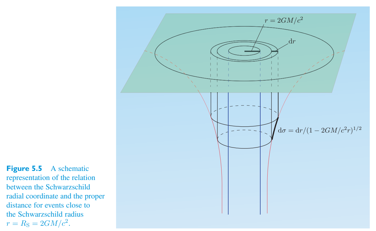
Exercise 5.4 Confirm that the proper distance around练习 5.4 确认周围的固有距离
a circle (proper C = 2 πr, according to circumference) in the \(\theta\) = \(\pi\)/2 plane centred at r = 0 is the Schwarzschild geometry.\(\theta\) = \(\pi\)/2 平面中以 r = 0 为中心的圆(根据周长,适当的 C = 2 πr)是史瓦西几何。
Proper distance固有距离
The Schwarzschild metric describes the spacetime around a static, spherically symmetric body as a set of nested spheres. The coordinate radius r of any one of those spheres can be determined by dividing its proper circumference by 2 \(\pi\).史瓦西度规将静态球对称物体周围的时空描述为一组嵌套球体。这些球体中任何一个的坐标半径 r 都可以通过将其固有周长除以 2 \(\pi\) 来确定。
Two events occurring at the same coordinate time and separated only by a radial coordinate distance d r will be separated by a proper radial distance在同一坐标时间发生且仅相隔径向坐标距离 d r 的两个事件将相隔适当的径向距离
5.4 Geodesic motion in Schwarzschild spacetime5.4 史瓦西时空中的测地运动
According to the geodesic principle discussed in Chapter 4, the time-like and null geodesics of a spacetime represent the possible world-lines of massive and massless particles moving under the influence of gravity alone. Remember, a world-line is a pathway through spacetime, not just a trajectory through space. So once we know the world-line of a freely falling particle — i.e. once we know the specific geodesic that it moves along — we know everything about that particular particle’s motion. In this section we examine some aspects of geodesic motion in the Schwarzschild spacetime around a static spherically symmetric body. We shall be particularly interested in motions relevant to astrophysics, so we shall be mainly concerned with orbital motion.根据第 4 章讨论的测地线原理,时空的类时测地线和零测地线代表了仅在引力影响下运动的有质量和无质量粒子的可能世界线。请记住,世界线是穿越时空的路径,而不仅仅是穿越空间的轨迹。因此,一旦我们知道了自由落体粒子的世界线,即一旦我们知道了它移动的特定测地线,我们就知道了关于该特定粒子运动的一切。在本节中,我们将研究史瓦西时空中围绕静态球对称体的测地运动的某些方面。我们将对与天体物理学相关的运动特别感兴趣,因此我们将主要关注轨道运动。
5.4.1 The geodesic equations5.4.1 测地线方程
As you saw in Chapters 3 and 4, the geodesics of a spacetime are usually presented as parameterized curves, represented by four coordinate functions x \(\mu\) (\(\lambda\)), where \(\lambda\) is an affine parameter that varies along the geodesic. The choice of parameter is not completely arbitrary. In the case of a massive particle moving along a time-like geodesic, the affine parameter is usually taken to be the proper time \(\tau\) that would be measured by a clock falling with the particle. It is also possible to use any linearly related parameter such as aτ + b, where a and b are constants, though this would be unusual. These choices are not possible for a null geodesic since d \(\tau\) = d s/c = 0 for each of its elements, so some other affine parameter must be adopted. In either case the parameter is chosen to be an affine parameter since this ensures that the coordinate functions will satisfy geodesic equations of the relatively simple form正如您在第 3 章和第 4 章中看到的,时空的测地线通常表示为参数化曲线,由四个坐标函数 x \(\mu\) (\(\lambda\)) 表示,其中 \(\lambda\) 是沿测地线变化的仿射参数。参数的选择并不是完全任意的。对于大质量粒子沿类时间测地线移动的情况,仿射参数通常被视为本征时间 \(\tau\),该时间由随粒子落下的时钟测量。也可以使用任何线性相关的参数,例如 aτ + b,其中 a 和 b 是常数,尽管这种情况并不常见。这些选择对于零测地线来说是不可能的,因为对于每个元素 d \(\tau\) = d s/c = 0,因此必须采用其他一些仿射参数。在任何一种情况下,参数都选择为仿射参数,因为这确保坐标函数满足相对简单形式的测地方程
where the Γ \(\mu\) \(\nu\)\(\rho\) are the connection coefficients that follow directly from the spacetime metric.其中 Γ \(\mu\) \(\nu\)\(\rho\) 是直接从时空度规得出的联络系数。
The general form of the non-zero connection coefficients was given in Section 5.1.2 at the start of the derivation of the Schwarzschild metric. Now that we know the explicit form of the Schwarzschild radius and the functions A (r) and B (r), we can write down the explicit form of all the non-zero connection coefficients:非零联络系数的一般形式在第 5.1.2 节史瓦西度规推导开始时给出。现在我们知道了史瓦西半径的显式形式以及函数 A (r) 和 B (r),我们可以写出所有非零联络系数的显式形式:
Using these connection coefficients, the geodesic equations provide the following four differential equations that must be satisfied by the four coordinate functions \(x^0\) = t (\(\lambda\)), \(x^1\) = r (\(\lambda\)), \(x_{2}\) = \(\theta\) (\(\lambda\)), \(x^{3}\) = \(\phi\) (\(\lambda\)) that describe any affinely parameterized geodesic in Schwarzschild spacetime:使用这些联络系数,测地方程提供了以下四个微分方程,必须由描述史瓦西时空中任何仿射参数化测地线的四个坐标函数 \(x^0\) = t (\(\lambda\))、\(x^1\) = r (\(\lambda\))、\(x_{2}\) = \(\theta\) (\(\lambda\))、\(x^{3}\) = \(\phi\) (\(\lambda\)) 来满足这些微分方程:
Given the initial location of a particle in Schwarzschild spacetime and the initial = d x \(\mu\)/d \(\lambda\), these four values of the four components of its tangent vector t \(\mu\) coupled, second-order, ordinary differential equations can be solved (numerically if not analytically) to determine the unique world-line of the particle. If the particle is massless, the magnitude of the initial tangent vector will be zero, showing the particle to be travelling at the speed of light, and the relevant world-line will turn out to be a null geodesic. For a particle with mass, the world-line will be a time-like geodesic.给定史瓦西时空中粒子的初始位置和初始 = d x \(\mu\)/d \(\lambda\),其切向量 t \(\mu\) 的四个分量的这四个值可以求解耦合的二阶常微分方程(如果不是解析的话,则以数值方式)以确定粒子的唯一世界线。如果粒子没有质量,则初始切向量的大小将为零,表明粒子以光速行进,并且相关的世界线将成为零测地线。对于具有质量的粒子,世界线将是一条类时间测地线。
As far as motion under gravity is concerned, the geodesic equations are the general relativistic analogues of Newton’s second law of motion. Both sets of equations may be expressed as differential equations, and their solution allows initial data to be used to predict subsequent motion. However, as you can see, the geodesic equations look formidable and can be very difficult to solve. Because of their difficulty we shall not attempt a direct solution in this case. There are simplifying techniques that can be used based on the Lagrangian approach introduced when we first derived the geodesic equations in Chapter 3, but those methods are beyond the level of this book. Instead, we shall take a lesson from Newtonian mechanics, where problems involving motion are often simplified by making use of constants of the motion such as energy and angular momentum.就引力运动而言,测地方程是牛顿第二运动定律的广义相对论类比。两组方程都可以表示为微分方程,并且它们的解允许使用初始数据来预测后续运动。然而,正如您所看到的,测地线方程看起来很复杂并且很难求解。由于它们的困难,我们不会在这种情况下尝试直接解决方案。基于我们在第 3 章中首次推导测地线方程时介绍的拉格朗日方法,可以使用一些简化技术,但这些方法超出了本书的范围。相反,我们应该从牛顿力学中吸取教训,其中涉及运动的问题通常通过利用运动常数(例如能量和角动量)来简化。
Exercise 5.5 Confirm the form of the first of the four练习 5.5 确认四个中第一个的形式
geodesic equations given above.上面给出的测地线方程。
5.4.2 Constants of the motion in Schwarzschild5.4.2 史瓦西运动常数
spacetime时空
To start, we recall that when geodesics were first introduced we described them as parameterized curves defined by x \(\mu\) (\(\lambda\)) with the particular property that the tangent vector d x \(\mu\)/d \(\lambda\) at any point remained parallel to itself under parallel transport. (This was a property that they shared with straight lines in a flat space.) Choosing the parameter \(\lambda\) to be an affine parameter ensures that as the tangent vector is transported along the geodesic, it not only remains self-parallel but also has a constant magnitude (more properly called a norm in this context). The square of that norm at every point on the geodesic is given by首先,我们回想一下,当测地线首次引入时,我们将它们描述为由 x \(\mu\) (\(\lambda\)) 定义的参数化曲线,其特殊属性是切向量 d x \(\mu\)/d \(\lambda\) 在任何点在平行传输下都保持与其自身平行。(这是它们与平坦空间中的直线共享的属性。)选择参数 \(\lambda\) 作为仿射参数可确保当切向量沿测地线传输时,它不仅保持自平行,而且具有恒定的大小(在这种情况下更准确地称为范数)。测地线上每一点的范数的平方由下式给出
and will be zero in the case of a null geodesic.在零测地线的情况下将为零。
If we regard the geodesic as the world-line of a massive particle and choose to use the proper time \(\tau\) (as measured by a clock falling with the particle) as the parameter \(\lambda\), then the tangent vector components d x \(\mu\)/d \(\lambda\) become d x \(\mu\)/d \(\tau\) and are seen to be the components of the particle’s four-velocity \([U^{\mu}]\). Now, for the four-velocity of a massive particle,如果我们将测地线视为大质量粒子的世界线,并选择使用本征时间 \(\tau\)(通过随粒子落下的时钟来测量)作为参数 \(\lambda\),则切向量分量 d x \(\mu\)/d \(\lambda\) 变为 d x \(\mu\)/d \(\tau\),并且可以视为粒子四速度的分量 \([U^{\mu}]\)。现在,对于大质量粒子的四速度,
So in this case the constant \(n^2\) in Equation 5.25 will be given by \(n^2\) = \(c^2\), and we can use our explicit knowledge of the Schwarzschild metric coefficients \(g_{\mu\nu}\) to expand Equation 5.25 as因此,在这种情况下,方程 5.25 中的常数 \(n^2\) 将由 \(n^2\) = \(c^2\) 给出,我们可以使用史瓦西度规系数 \(g_{\mu\nu}\) 的明确知识将方程 5.25 展开为
This still looks complicated, but apart from \(n^2\) = \(c^2\) there are four other constants of the motion that can help to simplify Equation 5.27. There are many ways of deducing these four conserved quantities, most of them drawing on the symmetry of the Schwarzschild solution. There are deep connections between symmetries and conservation laws throughout physics, so it is not surprising that the many symmetries of the Schwarzschild solution should give rise to conserved quantities in this case. In particular, we noted earlier that the static nature of the Schwarzschild solution indicates a symmetry associated with invariance under translation in time. This kind of symmetry is generally associated with the conservation of energy. Similarly, the solution’s invariance under rotations about the origin indicates spherical symmetry, and is associated with the conservation of angular momentum.这看起来仍然很复杂,但除了 \(n^2\) = \(c^2\) 之外,还有其他四个运动常数可以帮助简化方程 5.27。推导这四个守恒量的方法有很多,其中大多数都利用史瓦西解的对称性。在整个物理学中,对称性和守恒定律之间存在着深刻的联系,因此史瓦西解的许多对称性在这种情况下会产生守恒量也就不足为奇了。特别是,我们之前注意到史瓦西解的静态性质表明了与时间平移不变性相关的对称性。这种对称性通常与能量守恒有关。类似地,解在绕原点旋转下的不变性表明球对称性,并且与角动量守恒相关。
In the specific context of a freely falling body of non-zero mass m, moving along a time-like geodesic in Schwarzschild spacetime, the conserved quantity that plays the role of total energy (actually the energy per unit mass energy) is在非零质量 m 的自由落体在史瓦西时空中沿着类时测地线运动的特定背景下,扮演总能量(实际上是单位质量能量的能量)的守恒量为
When dealing with the analogue of angular momentum, which is a vector, there are three conserved scalar quantities. These are most conveniently regarded as the magnitude of the angular momentum per unit mass, J/m, and two angles that determine the direction of the angular momentum vector. In practice, rather than dealing with whatever direction the angular momentum actually has, it is usually easier to transform the coordinates so that the angular momentum points along the polar axis, with the consequence that the motion is confined to the plane in which当处理角动量的类似物(矢量)时,存在三个守恒标量。这些最方便地被视为每单位质量角动量的大小,J/m,以及确定角动量矢量方向的两个角度。在实践中,与处理角动量实际具有的任何方向相比,通常更容易变换坐标,使角动量沿着极轴指向,结果是将运动限制在其中的平面内。
\(\theta\) = \(\pi\)/2 and consequently d \(\theta\)/d t = 0. So, without any real loss of generality, two of the three constants of the motion associated with angular momentum are represented by the single condition\(\theta\) = \(\pi\)/2,因此 d \(\theta\)/d t = 0。因此,在不失一般性的情况下,与角动量相关的三个运动常数中的两个由单个条件表示
while the third turns out to be而第三个结果是
Take care to note that the quantities \(E/(mc^2)\) and J/m are specific to the Schwarzschild metric; they do not represent general definitions that can automatically be applied to other cases. If we now use Equations 5.28, 5.29 and 5.30 to simplify Equation 5.27, we see that请注意,数量 \(E/(mc^2)\) 和 J/m 特定于史瓦西度规;它们并不代表可以自动应用于其他情况的一般定义。如果我们现在使用方程 5.28、5.29 和 5.30 来简化方程 5.27,我们会看到
Rearranging this gives重新排列这给出
This equation, which already incorporates the general relativistic analogues of energy conservation and angular momentum conservation, describes the changes in the radial position coordinate with proper time for a freely falling \(\theta\) = \(\pi\)/2. The phrase particle of non-zero mass moving in the equatorial plane ‘freely falling’ can give the impression that the particle is plummeting radially inwards towards the central body. That is a possible form of freely falling motion, but not the only one. All ‘freely falling’ really means is that the motion is determined by gravity alone. In this sense the Moon is (very nearly) freely falling around the Earth and the Earth is (very nearly) freely falling around the Sun. So Equation 5.32 holds the key to describing orbital motion about the central massive body in Schwarzschild spacetime, and that is how we shall use it in the next subsection. Before doing that, however, let’s see how Equation该方程已经包含了能量守恒和角动量守恒的广义相对论类比,描述了自由落体 \(\theta\) = \(\pi\)/2 的径向位置坐标随固有时间的变化。在赤道平面上运动的非零质量粒子“自由落体”这一短语给人的印象是粒子正在径向向内朝中心体垂直下落。这是自由落体运动的一种可能形式,但不是唯一的形式。所有“自由落体”的真正含义是运动仅由引力决定。从这个意义上说,月球(非常接近)围绕地球自由落体,地球(非常接近)围绕太阳自由落体。因此,方程 5.32 是描述史瓦西时空中中心大质量天体轨道运动的关键,这就是我们在下一小节中将如何使用它的方法。然而,在此之前,让我们看看方程如何
5.32 together with5.32 连同
the definitions contained in Equations 5.28 and 5.30 can be used to solve a problem involving purely radial motion.方程 5.28 和 5.30 中包含的定义可用于解决涉及纯径向运动的问题。
Worked Example 5.1工作示例 5.1
Show that in Schwarzschild spacetime, the motion of a test particle in radial free fall (i.e. directly towards r = 0) satisfies the relation证明在史瓦西时空中,测试粒子的径向自由落体运动(即直接朝向 r = 0)满足以下关系
Solution解决方案
To determine the equation of motion for a freely falling body travelling along a radial geodesic, we can use Equation 5.32, together with the supplementary Equations 5.28 and 5.30 that define E and J. In the case of purely radial motion \(\phi\) is constant, so d \(\phi\)/d \(\tau\) = 0, so Equation 5.30 shows that J = 0. Equation 5.32 therefore reduces to为了确定沿径向测地线运动的自由落体物体的运动方程,我们可以使用方程 5.32,以及定义 E 和 J 的补充方程 5.28 和 5.30。在纯径向运动的情况下,\(\phi\) 是常数,因此 d \(\phi\)/d \(\tau\) = 0,因此方程 5.30 显示 J = 0。因此,方程 5.32 简化为
Differentiating with respect to \(\tau\) gives对 \(\tau\) 求导可得出
and dividing through by d r/d \(\tau\) gives除以 d r/d \(\tau\) 得到
as required.根据需要。
The result that has just been derived in this worked example looks very much like the corresponding Newtonian result for free fall under the gravitational pull of a spherically symmetric mass in Euclidean space. Note, however, the several differences between the general relativistic result and its Newtonian counterpart. In the first place, talking about free fall under gravity is fine in general relativity, but talking of the ‘pull’ of gravity or gravitational ‘attraction’ would be quite wrong since there is no gravitational ‘force’ in general relativity, and even the term gravitational ‘field’ only retains a meaning when interpreted in terms of the metric coefficients, which can vary from place to place. Similarly, the Newtonian result directly relates the second derivative of the radial distance with respect to time to the inverse square of the radial distance, but in the general relativistic result the second derivative is with respect to proper time \(\tau\), and r is the coordinate distance, not the ‘physical’ proper distance. In the Newtonian limit, when d r/d \(\tau\) (c and the particle is sufficiently far from the spherical mass for the field to be weak, these differences vanish, and the general relativistic result does reduce to the Newtonian result. This shows how Einstein’s theory of motion under gravity encompasses Newton’s theory and reduces to it under appropriate conditions. Nonetheless, away from the Newtonian limit, especially when close to the Schwarzschild radius, the differences are real and significant.在这个工作示例中刚刚得出的结果看起来非常类似于欧几里德空间中球对称质量的引力作用下自由落体的相应牛顿结果。然而,请注意广义相对论结果与其牛顿对应结果之间的一些差异。首先,在广义相对论中谈论引力下的自由落体是可以的,但是谈论引力的“拉力”或引力“吸引力”就大错特错了,因为广义相对论中不存在引力“力”,甚至引力“场”这个术语也只有在用度规系数解释时才保留意义,而度规系数可能因地而异。类似地,牛顿结果直接将径向距离对时间的二阶导数与径向距离的平方反比联系起来,但在广义相对论结果中,二阶导数是相对于固有时间τ的,r是坐标距离,而不是“物理”固有距离。在牛顿极限下,当 d r/d \(\tau\) (c 和粒子距离球形质量足够远,场很弱时,这些差异消失,广义相对论结果确实还原为牛顿结果。这表明爱因斯坦的引力运动理论如何包含牛顿理论,并在适当的条件下还原为牛顿理论。尽管如此,远离牛顿极限,尤其是接近史瓦西半径时,差异是真实且显着的。
To summarize, we have the following.总而言之,我们有以下几点。
Freely falling motion in Schwarzschild spacetime史瓦西时空中的自由落体运动
The motion of a particle of mass m falling freely in the \(\theta\) = \(\pi\)/2 plane of a Schwarzschild spacetime is described by the radial motion equation质量为 m 的粒子在史瓦西时空 \(\theta\) = \(\pi\)/2 平面中自由落体的运动由径向运动方程描述
where \(\tau\) is the proper time as would be measured by a clock falling with the particle, and the constants of the motion, \(E/(mc^2)\) and J/m, the Schwarzschild analogues of energy per unit mass energy and angular momentum magnitude per unit mass, are determined by其中 \(\tau\) 是通过与粒子一起下落的时钟测量的本征时间,运动常数 \(E/(mc^2)\) 和 J/m(单位质量能量的史瓦西类似物)由下式确定:
5.4.3 Orbital motion in Schwarzschild spacetime5.4.3 史瓦西时空中的轨道运动
The shape of an orbit in the \(\theta\) = \(\pi\)/2 plane of Schwarzschild spacetime is described by expressing r as a function of \(\phi\). In the previous subsection we developed a differential equation relating r to \(\tau\); we now need to convert that into a tractable relation between r and \(\phi\), and then investigate its solution. We start by noting that史瓦西时空 \(\theta\) = \(\pi\)/2 平面中的轨道形状通过将 r 表示为 \(\phi\) 的函数来描述。在上一小节中,我们开发了一个将 r 与 \(\tau\) 相关的微分方程;我们现在需要将其转换为 r 和 \(\phi\) 之间的易于处理的关系,然后研究其解决方案。我们首先注意到
\(\theta\) = \(\pi\)/2, to eliminate and then use the fact that J/m = \(r^2\) d \(\phi\)/d \(\tau\), in the plane d \(\phi\)/d \(\tau\), giving\(\theta\) = \(\pi\)/2,消除然后使用 J/m = \(r^2\) d \(\phi\)/d \(\tau\),在平面 d \(\phi\)/d \(\tau\) 中,给出
Substituting this result into Equation 5.32 gives将此结果代入公式 5.32 得出
Now we apply a standard ‘trick’ of orbital analysis by introducing the reciprocal variable u = 1/r, and rewrite this equation as现在我们通过引入倒数变量 u = 1/r 来应用轨道分析的标准“技巧”,并将该方程重写为
equation by d u/d \(\phi\) Differentiating with respect to \(\phi\) and dividing the resulting gives the orbital shape equation that we need.方程 d u/d \(\phi\) 对 \(\phi\) 进行微分并除以所得结果即可得到我们需要的轨道形状方程。
Orbital shape equation轨道形状方程
It is informative to compare this result with the analogous result from Newtonian mechanics for orbits around a massive spherically symmetric body. In the Newtonian case the result is将该结果与围绕巨大球对称体的轨道的牛顿力学的类似结果进行比较是非常有用的。在牛顿情况下,结果是
This is the same as the Schwarzschild expression, apart from the absence of the final relativistic term 3 GM \(u^{2}\)/\(c^2\). That additional term will vanish in the limit as u approaches zero, showing that as long as r is sufficiently large, the Newtonian orbits will be recovered from the relativistic orbit equation, as they should be. Of course, for ‘small’ values of r (meaning close to 2 GM/\(c^2\)), the value of u will be large and the additional term will not be negligible. There will then be significant differences between the Newtonian and relativistic behaviours.除了缺少最后的相对论项 3 GM \(u^{2}\)/\(c^2\) 之外,这与史瓦西表达式相同。当 u 接近零时,附加项将在极限中消失,这表明只要 r 足够大,牛顿轨道就会从相对论轨道方程中恢复,正如它们应该的那样。当然,对于 r 的“小”值(意味着接近 2 GM/\(c^2\)),u 的值会很大,并且附加项将不可忽略。牛顿行为和相对论行为之间将会存在显着差异。
Additional insight into the behaviour of orbits comes from a study of energy, so it is useful here to rewrite the radial motion equation (Equation 5.32) that we developed in the previous subsection in a way that emphasizes the role of energy:对轨道行为的更多了解来自对能量的研究,因此这里重写我们在上一小节中开发的径向运动方程(方程 5.32)是有用的,以强调能量的作用:
The quantity on the left is not an energy, but for a particle of given mass it is determined by the orbital energy. The expression on the right consists of a ‘kinetic’ term (proportional to (d r/d \(\tau\)) 2) added to a sum of terms that depend only on r for given values of J and m. This is sufficient to earn the sum of those dependent terms the name ‘effective potential’ and the symbol V eff. Thus we can write左边的量不是能量,但对于给定质量的粒子,它由轨道能量决定。右侧的表达式包含一个“动力学”项(与 (d r/d \(\tau\)) 2 成比例),添加到仅依赖于给定 J 和 m 值的 r 的项之和。这足以获得这些从属术语“有效电势”名称和符号 V eff 的总和。因此我们可以写
where在哪里
Now, a very similar equation arises in Newtonian orbital analysis, where the constant orbital energy E Newton is given by现在,牛顿轨道分析中出现了一个非常相似的方程,其中恒定轨道能量 E Newton 由下式给出
with和
The Newtonian and Schwarzschild effective potentials for a positive value of J are shown in Figure 5.6. In the Newtonian case the angular momentum magnitude J is the source of an infinite ‘effective potential barrier’ that prevents particles with non-zero angular momentum magnitude from reaching r = 0. In the Schwarzschild case the behaviour at small values of r is quite different. Indeed, for sufficiently small values of J there is no barrier at all.J 为正值时的牛顿和史瓦西有效势如图 5.6 所示。在牛顿情况下,角动量大小 J 是无限“有效势垒”的来源,它阻止具有非零角动量大小的粒子达到 r = 0。在史瓦西情况下,r 值较小时的行为完全不同。事实上,对于足够小的 J 值来说,根本不存在障碍。
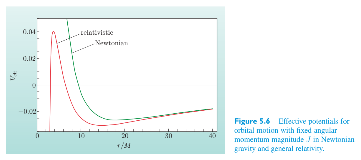
The difference between the Newtonian and Schwarzschild effective potentials comes from the extra term − GM J 2/\(m^{2}\) \(c^2\) \(r^3\) in the Schwarzschild case. One of the \(\theta\) = \(\pi\)/2 plane. This its effects is to cause the orbits of particles to rotate in effect is negligible at large values of r but significant for small values, preventing elliptical orbits from closing and causing them to follow the kind of rosette pattern shown in Figure 5.7. This is another effect with astronomically observable consequences to which we shall return in Chapter 7.牛顿有效势和史瓦西有效势之间的差异来自于额外项 - 史瓦西案例中的 GM J 2/\(m^{2}\) \(c^2\) \(r^3\)。 \(\theta\) = \(\pi\)/2 平面之一。它的作用是导致粒子轨道旋转,在 r 值较大时,效果可以忽略不计,但在 r 值较小时,效果很显着,防止椭圆轨道闭合并导致它们遵循图 5.7 中所示的玫瑰花图案。这是另一种具有天文学上可观察到的后果的效应,我们将在第七章中再次讨论。
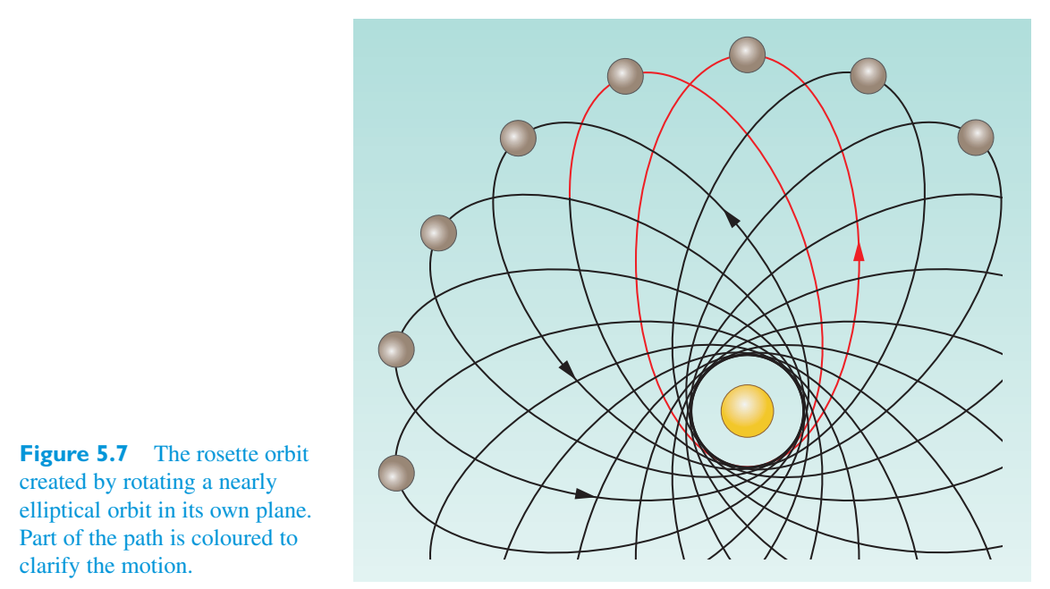
Exercise 5.6 Both Newtonian and Schwarzschild orbital练习 5.6 牛顿轨道和史瓦西轨道
dynamics allow stable circular orbits to exist at large values of r, but in the Schwarzschild case there is a √ lower limit to the radius of a stable circular orbit that corresponds to J/m = 2 3 GM/c.动力学允许在较大的 r 值下存在稳定的圆形轨道,但在史瓦西情况下,稳定圆形轨道的半径存在 √ 下限,对应于 J/m = 2 3 GM/c。
(a) What is the (coordinate) radius of that orbit?(a) 该轨道的(坐标)半径是多少?
(b) What is the corresponding value of the parameter E?(b) 参数E对应的值是多少?
Summary of Chapter 5第 5 章总结
1. The Schwarzschild metric tensor is1. 史瓦西度规张量为
though the term ‘Schwarzschild metric’ is more often applied as the corresponding line element尽管术语“史瓦西度规”更常用作相应的线元素
2. The Schwarzschild metric coefficients provide a solution of the Einstein2. 史瓦西度规系数提供了爱因斯坦方程的解
vacuum field equations R \(\mu\)\(\nu\) − \(g_{\mu\nu}\) R/2 = 0 in the empty region of spacetime surrounding a non-rotating spherically symmetric body of fixed mass M.真空场方程 R \(\mu\)\(\nu\) − \(g_{\mu\nu}\) R/2 = 0 在围绕固定质量 M 的非旋转球对称体的时空区域中。
3. The solution is spherically symmetric (having the invariance of a spherical3. 该解是球对称的(具有球面的不变性)
shell), asymptotically flat (approaching the Minkowski metric in spherical polar coordinates at large r), stationary (having metric coefficients that are time-independent) and static (having a line element that is invariant under time reversal).壳)、渐近平坦(在大 r 处接近球极坐标中的闵可夫斯基度规)、平稳(具有与时间无关的度规系数)和静态(具有在时间反转下不变的线元素)。
4. The solution is singular, approaching infinity as r → \(R_S\) = 2 GM/\(c^2\), the4. 解是奇异的,当 r → \(R_S\) = 2 GM/\(c^2\) 时接近无穷大,
Schwarzschild radius, and as r → 0. The first of these is a coordinate singularity that can be transformed away by an appropriate choice of coordinates; the second is a gravitational singularity that is present in curvature-related invariants and cannot be transformed away. Neither singularity is within the region described by the solution for normal ‘star-like’ bodies.史瓦西半径,并且 r → 0。第一个是坐标奇点,可以通过适当选择坐标来转换;第二个是引力奇点,它存在于曲率相关的不变量中并且无法被转化掉。两个奇点都不在正常“类星”天体解所描述的区域内。
5. The solution has great generality, Birkhoff’s theorem showing that it applies5. 该解具有很强的通用性,伯克霍夫定理表明它适用
to the exterior region of any distribution of energy and momentum characterized by mass M that produces purely isotropic effects in that region.到以质量 M 为特征的任何能量和动量分布的外部区域,在该区域中产生纯各向同性效应。
6. The Schwarzschild coordinates t, r, \(\theta\), \(\phi\) lack immediate metrical6. 史瓦西坐标 t, r, \(\theta\), \(\phi\) 缺乏直接度规
significance. Infinitesimal differences in coordinate time (d t) and coordinate radial distance (d r) may be related to infinitesimal differences in measurable proper time (d \(\tau\)) and measurable proper distance (d \(\sigma\)) using the Schwarzschild metric. Finite intervals of proper time and proper distance may be determined by performing appropriate integrals involving the infinitesimal intervals.意义。坐标时间(d t) 和坐标径向距离(d r) 中的无穷小差异可能与使用史瓦西度规的可测量固有时间(d \(\tau\)) 和可测量固有距离(d \(\sigma\)) 中的无穷小差异相关。本征时间和固有距离的有限间隔可以通过执行涉及无穷小间隔的适当积分来确定。
7. When considering observations of events in general relativity, the location of7. 当考虑广义相对论中的事件观测时,
the observer is significant as well as the observer’s state of motion. When considering events in Schwarzschild spacetime, three observers are commonly mentioned; a local stationary observer at fixed Schwarzschild coordinates, a local freely falling observer, and a distant observer (at r = ∞), who may be regarded as freely falling while stationary and whose own ‘local’ observations concern sightings of the events.观察者以及观察者的运动状态都很重要。当考虑史瓦西时空中的事件时,通常会提到三个观察者:固定史瓦西坐标上的本地静止观察者、本地自由落体观察者和远处观察者(在 r = ∞ 处),后者可以被视为静止时自由落体,并且其自己的“本地”观察涉及事件的目击。
8. Physical meaning can be associated with Schwarzschild coordinates based8. 物理意义可以与基于史瓦西坐标的
on the observations that (a) the difference in coordinate time between two events at the same coordinate position is equal to the measurable proper time between sightings of those events by a stationary observer at infinity, and (b) a circle centred on the origin with fixed coordinate radius r has the measurable proper circumference C = 2 πr.观察结果如下:(a) 同一坐标位置上两个事件之间的坐标时间差等于无穷远静止观察者两次观测到这些事件之间的可测量固有时间,以及 (b) 以原点为中心、坐标半径为 r 的圆具有可测量固有周长 C = 2 πr。
9. Two events that occur at the same coordinate time and with the same angular9. 同一坐标时间、同一角度发生的两个事件
coordinates, but separated by a coordinate radial distance d r will, according to a local stationary observer, be separated by a proper distance坐标,但相隔坐标径向距离 d r 根据本地静止观察者,将相隔固有距离
Similarly, two events that occur at the same coordinate position but separated by coordinate time interval d t will, according to a local stationary observer, be separated by a proper time类似地,发生在同一坐标位置但相隔坐标时间间隔 d t 的两个事件,根据本地静止观察者的观点,将相隔适当的时间
10. Due to gravitational time dilation, a clock at rest at10. 由于引力时间膨胀,时钟静止在
radial coordinate r, with ticks of proper duration d \(\tau\) r, will be seen to have ticks of longer duration d \(\tau\) = d \(\tau\)/(1 − 2 GM/rc 2) 1/2 by a stationary distant observer. This implies the existence of an observable gravitational redshift in which a source emitting radiation of proper frequency \(f_{\rm em}\) located at fixed radial coordinate \(r_{\rm em}\) is seen by a stationary distant observer to have frequency径向坐标 r,具有适当持续时间 d \(\tau\) r 的刻度,对于静止的远处观察者来说,将看到具有较长持续时间 d \(\tau\) = d \(\tau\)/(1 − 2 GM/rc 2) 1/2 的刻度。这意味着存在可观测的引力红移,其中位于固定径向坐标 \(r_{\rm em}\) 的发射适当频率 \(f_{\rm em}\) 的辐射的源被静止的远距离观察者看到具有频率
11. Equations describing the possible world-lines of freely11. 描述自由可能的世界线的方程
falling massive and massless particles as time-like and null geodesics may be deduced from the geodesic equations applied to Schwarzschild spacetime. The world-line of a specific particle will be determined by the initial position and velocity of that particle. However, for the study of orbital motion it is simpler to consider the quantities that represent constants of the motion, including the norm of the tangent vector, the (generalized) orbital energy and the (generalized) orbital angular momentum.落下的大质量和无质量粒子作为类时测地线和零测地线可以从应用于史瓦西时空的测地线方程推导出来。特定粒子的世界线将由该粒子的初始位置和速度决定。然而,对于轨道运动的研究,更简单的是考虑表示运动常数的量,包括切向量的范数、(广义)轨道能量和(广义)轨道角动量。
12. For a freely falling particle of mass m following a12. 对于质量为 m 的自由落体粒子,遵循
geodesic parameterized by the proper time \(\tau\) (as measured by a co-moving freely falling clock), the conserved total orbital energy per unit mass energy is \(E/(mc^2)\) = (1 − 2 GM/\(c^2\) r)(d t/d \(\tau\)) and the conserved orbital angular \(\sin^2 \theta\) (d \(\phi\)/d \(\tau\)). In the momentum magnitude per unit mass is J/m = \(r^2\) case of motion in the equatorial plane (\(\theta\) = \(\pi\)/2), the radial motion is described by由原时 \(\tau\) 参数化的测地线(由共动自由落体时钟测量),每单位质量能量守恒的总轨道能量为 \(E/(mc^2)\) = (1 − 2 GM/\(c^2\) r)(d t/d \(\tau\)) 和守恒轨道角 \(\sin^2 \theta\) (d \(\phi\)/d \(\tau\))。在每单位质量的动量大小为 J/m = \(r^2\) 的情况下,在赤道平面内运动 (\(\theta\) = \(\pi\)/2),径向运动由下式描述
variable u = 1/r by while the orbital shape is described using the reciprocal变量 u = 1/r by 而轨道形状则使用倒数来描述
13. At large values of r, far from the central body, the13. 当 r 值较大且远离中心体时,
orbits of massive particles approach their Newtonian analogues. At smaller values of r, differences from Newtonian behaviour include the absence of an ‘angular momentum barrier’ preventing particles with non-zero angular momentum magnitude from reaching r = 0, the absence of stable circular orbits with r < 6 GM/\(c^2\), and the failure of ‘elliptical’ orbits to close due to a rotation of the ellipse in the orbital plane. These differences can be associated with the action of an additional term in the Schwarzschild ‘effective potential’ that governs the radial motion in the relativistic case.大质量粒子的轨道接近牛顿的类似物。在 r 值较小时,与牛顿行为的差异包括不存在阻止角动量大小非零的粒子达到 r = 0 的“角动量势垒”、不存在 r < 6 GM/\(c^2\) 的稳定圆形轨道,以及由于椭圆在轨道平面中的旋转而导致“椭圆”轨道无法闭合。这些差异可能与史瓦西“有效势”中的附加项的作用有关,该项控制相对论情况下的径向运动。
Chapter 6 Black holes第6章黑洞
Introduction介绍
Black holes are believed to be among the most exotic objects in the Universe. They are regions of spacetime distorted by the gravitational effects of bodies such as collapsed stars to such an extent that light itself is unable to escape.黑洞被认为是宇宙中最奇异的物体之一。它们是被坍缩恒星等物体的引力效应扭曲的时空区域,扭曲到光本身无法逃逸的程度。
The study of black holes and their associated astrophysical properties has become an enormous subject. In this chapter we shall address only some of the key points. We start with a wide-ranging section that contains some basic definitions, a brief history of the subject, and a classification of the various types of black hole. We then devote one section to non-rotating black holes and another to rotating black holes. Finally, in Section 6.4, we go beyond the ‘classical’ black holes of general relativity to discuss some possible implications of quantum physics for black holes, particularly the proposal that quantum physics allows black holes to be sources of radiation. Throughout the discussion there will be references to possible astronomical evidence of black holes, but that subject will be further discussed in Chapter 7, which concerns the testing of general relativity by experiment and observation.对黑洞及其相关天体物理特性的研究已成为一个巨大的课题。在本章中,我们将仅讨论一些关键点。我们从一个内容广泛的部分开始,其中包含一些基本定义、主题简史以及各种类型黑洞的分类。然后,我们将一部分用于非旋转黑洞,另一部分用于旋转黑洞。最后,在第 6.4 节中,我们超越广义相对论的“经典”黑洞,讨论量子物理学对黑洞的一些可能的影响,特别是量子物理学允许黑洞成为辐射源的提议。在整个讨论过程中,将会提到黑洞可能存在的天文学证据,但该主题将在第七章中进一步讨论,该章涉及通过实验和观察来检验广义相对论。
6.1 Introducing black holes6.1 黑洞介绍
The term ‘black hole’ was not introduced until the 1960s, though the basic concept can be traced back much further and has its roots in the Schwarzschild solution that was introduced in the previous chapter. We shall begin with some informal definitions and a brief historical survey that will trace the tangled history and even the pre-history of black holes.“黑洞”这个术语直到 20 世纪 60 年代才被引入,尽管其基本概念可以追溯到更远的地方,并且根源于上一章介绍的史瓦西解。我们将从一些非正式的定义和简短的历史调查开始,追溯黑洞的复杂历史,甚至史前史。
6.1.1 A black hole and its event horizon6.1.1 黑洞及其事件视界
In general relativity, a black hole is a region of spacetime that matter and radiation may enter but from which they cannot escape. It’s a ‘hole’ because matter and radiation can fall into it. It’s ‘black’ because light is unable to escape from it.在广义相对论中,黑洞是物质和辐射可以进入但无法逃脱的时空区域。这是一个“洞”,因为物质和辐射可以落入其中。它是“黑”的,因为光无法从它逸出。
Note that a black hole is essentially a spacetime structure, not a material one. This makes it very different from more familiar astronomical bodies, such as stars and planets, which are primarily composed of matter. Also note that our characterization of a black hole implies that it must be bounded by some kind of closed surface that will allow light to enter, but not to leave again. This light-trapping ‘one-way’ surface is called an event horizon and will feature prominently in the discussions that follow.请注意,黑洞本质上是一种时空结构,而不是物质结构。这使得它与主要由物质组成的恒星和行星等更熟悉的天体非常不同。另请注意,我们对黑洞的描述意味着它必须受到某种封闭表面的限制,该封闭表面将允许光线进入,但不会再次离开。这种捕光的“单向”表面被称为事件视界,并将在接下来的讨论中占据重要地位。
In the case of the simplest kind of black hole, which is described by the Schwarzschild metric, the event horizon is located at the Schwarzschild radius r = \(R_S\) = 2 GM/\(c^2\) and may be thought of as a sphere, though it follows from what was said about coordinates and distances in the previous chapter that 2 GM/\(c^2\) is its coordinate radius, not its proper (physical) radius.在用史瓦西度规描述的最简单的黑洞的情况下,事件视界位于史瓦西半径 r = \(R_S\) = 2 GM/\(c^2\) 处,并且可以被认为是一个球体,尽管从上一章中关于坐标和距离的内容可以得出,2 GM/\(c^2\) 是其坐标半径,而不是其正确的(物理)半径。
6.1.2 A brief history of black holes6.1.2 黑洞简史
Although the term ‘black hole’ took a long time to emerge, the story of black holes begins with the birth of general relativity and the Schwarzschild solution, both of which were published in 1916. However, long before that, in the context of Newtonian gravitation, there had already been speculations about the possibility of ‘dark stars’ — material bodies so dense that light would be unable to escape from them. The thinking behind this proposal was simple. If a projectile of mass m is launched from the surface of a spherical body of mass M and radius R, then in order to escape from the gravitational influence of that body the projectile must gain gravitational potential energy GM m/R. If this energy is to come from the projectile’s initial kinetic energy at the time of launch, then the required launch speed, sometimes referred to as the escape虽然“黑洞”一词的出现很久了,但黑洞的故事却始于广义相对论和史瓦西解的诞生,两者均于 1916 年发表。然而,早在这之前,在牛顿引力的背景下,就已经有人猜测“暗星”的可能性,这种物质的密度如此之大,以至于光无法从它们中逃逸。这个提议背后的想法很简单。如果从质量为 M、半径为 R 的球体表面发射质量为 m 的抛射体,那么为了摆脱该球体的引力影响,抛射体必须获得引力势能 GM m/R。如果该能量来自弹丸发射时的初始动能,则所需的发射速度,有时称为逃逸速度
The projectile mass m cancels, so the escape speed, independent of projectile mass, is弹丸质量 m 抵消,因此与弹丸质量无关的逃逸速度为
It follows from this that the escape speed v es will be greater than the speed of light c if the radius and mass of the body are related by由此可见,如果物体的半径和质量之间存在以下关系,则逃逸速度 es 将大于光速 c
Such a body, it was speculated, would trap light and would therefore be dark.据推测,这样的物体会捕获光线,因此会是黑暗的。
These ideas, introduced independently by John Michell (1724–1793) and Pierre-Simon Laplace (1749–1827) in the eighteenth century, have very little to do with the black holes of general relativity, but they do show that the physical concept of gravitational light trapping is not new.这些想法由约翰·米歇尔(John Michell,1724-1793)和皮埃尔-西蒙·拉普拉斯(Pierre-Simon Laplace,1749-1827)在十八世纪独立提出,与广义相对论的黑洞关系不大,但它们确实表明引力光捕获的物理概念并不新鲜。
That idea was implicit in Schwarzschild’s solution when it was developed in 1915, though that was not properly appreciated at the time. In fact, the familiar form of the Schwarzschild solution,当史瓦西的解决方案于 1915 年提出时,这个想法就隐含在其中,尽管当时并没有得到适当的重视。事实上,史瓦西解的常见形式,
was introduced about a year later by the mathematician David Hilbert (1862–1943), but even this did not make clear the physical behaviour associated with events at r = 2 GM/\(c^2\). Additionally, the Schwarzschild radius of real bodies (3 km for a body with the mass of the Sun) was thought to be too small to be of any physical significance, so its physical nature did not receive much attention.大约一年后,数学家戴维·希尔伯特(David Hilbert,1862-1943)提出了这一理论,但即使如此,也没有阐明与 r = 2 GM/\(c^2\) 时的事件相关的物理行为。此外,真实物体的史瓦西半径(太阳质量的物体为3公里)被认为太小,不具有任何物理意义,因此其物理性质没有受到太多关注。
- ● Regarding the Earth (total mass \(5.97\times10^{24}\) kg) as● 将地球(总质量\(5.97\times10^{24}\) kg)视为
a spherically symmetric body, what is its Schwarzschild radius?球对称体,它的史瓦西半径是多少?
❍ For the Earth, × \(10^{24}\)/(\(9.00\times10^{16}\)) m❍ 对于地球来说,× \(10^{24}\)/(\(9.00\times10^{16}\)) m
= \(8.84\times10^{-3}\) m,= \(8.84\times10^{-3}\)米,
or about 9 mm.或约9毫米。
It was pointed out during the 1920s that not all singularities in the metric \(g_{\mu\nu}\) are physically significant; they could be a consequence of the coordinates being used rather than the physics being described. This opened up the possibility that bodies might be able to undergo a complete gravitational collapse, shrinking to a point of infinite density irrespective of any singular surfaces that got in their way, provided that those singularities were entirely due to the choice of coordinates. In the case of a spherically symmetric body, surrounded by empty space described by the Schwarzschild metric, the singularity associated with r = \(R_S\) was eventually recognized as being a coordinate singularity, but this knowledge was slow to spread and the belief that the singularity was physical remained common at least until the late 1930s. In any case, planets were not sufficiently dense to undergo a complete gravitational collapse; the electrical repulsion between the atoms that they contained was sufficient to balance the gravitational tendency to collapse. Normal stars, such as the Sun, were also resistant to gravitational collapse. The plasma at the centre of the Sun is believed to be roughly ten times denser than lead, but even at these densities the thermal pressure resulting from energy releasing nuclear reactions (together with a contribution from radiation pressure) is sufficient to guarantee a star’s equilibrium with a radius in the order of a million kilometres.20 世纪 20 年代有人指出,并非度规 \(g_{\mu\nu}\) 中的所有奇点都具有物理意义;它们可能是所使用的坐标的结果,而不是所描述的物理原理的结果。这开启了一种可能性,即物体可能能够经历完全的引力塌缩,收缩到无限密度的点,而不管任何阻碍它们的奇点表面,只要这些奇点完全是由于坐标的选择造成的。在球对称体的情况下,周围环绕着史瓦西度规所描述的真空,与 r = \(R_S\) 相关的奇点最终被认为是坐标奇点,但这种知识传播缓慢,并且至少直到 20 世纪 30 年代末,奇点是物理奇点的信念仍然很普遍。无论如何,行星的密度不足以承受完全的引力塌缩。它们所含原子之间的电斥力足以平衡引力塌缩的趋势。普通恒星,例如太阳,也能抵抗引力塌缩。据信,太阳中心的等离子体密度大约是铅的十倍,但即使在这样的密度下,释放能量的核反应所产生的热压力(加上辐射压力的贡献)也足以保证半径约为一百万公里的恒星的平衡。
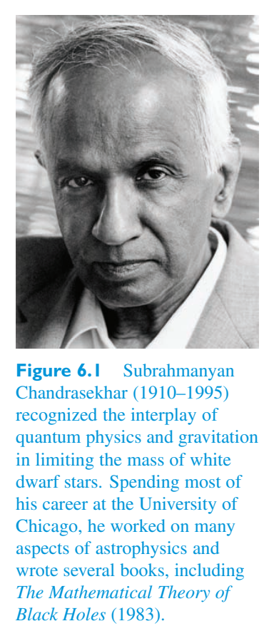
The astrophysics of highly evolved stellar bodies, in which nuclear reactions have ceased due to a lack of fuel, became a major topic in the 1930s. It had been suggested in the mid-1920s that the small dense stars known as white dwarf stars were supported against gravitational collapse by a degeneracy pressure arising from the quantum physics of the electrons that they contained. This idea was taken up by Subrahmanyan Chandrasekhar (Figure 6.1), an Indian theorist studying at the University of Cambridge. In 1931 he proposed that there was an upper limit (about 1.4 times the mass of the Sun) to the mass of any white dwarf supported by electron degeneracy pressure. If the star’s mass exceeded that limit, gravity would overwhelm the degeneracy pressure and a gravitational collapse would ensue. Some were doubtful about Chandrasekhar’s ideas, most notably the Cambridge-based astrophysicist Sir Arthur Eddington (1882–1944), who had been responsible for much of the foundational work on the internal constitution of stars. Working in the same university, Chandrasekhar came to know Eddington well and admired his work; Eddington’s opposition was a professional and personal blow that caused Chandrasekhar to abandon his work on white dwarfs and move to the USA, though his ideas are now an accepted part of astrophysical theory and his insight was eventually rewarded with a Nobel prize for physics.高度演化的恒星体的天体物理学(其中核反应由于缺乏燃料而停止)成为 20 世纪 30 年代的一个主要话题。 20 年代中期有人提出,被称为白矮星的小型致密恒星受到其所含电子的量子物理产生的简并压力的支持,免于引力塌缩。这个想法被剑桥大学的印度理论家 Subrahmanyan Chandrasekhar(图 6.1)采纳。 1931年,他提出电子简并压力支持的任何白矮星的质量都有一个上限(大约是太阳质量的1.4倍)。如果恒星的质量超过这个极限,引力就会压倒简并压力,从而发生引力塌缩。有些人对钱德拉塞卡的想法表示怀疑,其中最著名的是剑桥的天体物理学家阿瑟·爱丁顿爵士(Arthur Eddington,1882-1944 年),他负责恒星内部构成的大部分基础工作。在同一所大学工作时,钱德拉塞卡逐渐了解爱丁顿并钦佩他的工作。爱丁顿的反对是对职业和个人的打击,导致钱德拉塞卡放弃了他在白矮星方面的工作并移居美国,尽管他的想法现在已被天体物理理论所接受,并且他的洞察力最终获得了诺贝尔物理学奖。
Another development came in 1932, the year in which the neutron was discovered. Very soon after hearing of the discovery, the Russian theoretical physicist Lev Landau (1908–1968) suggested the possibility of neutron stars, the outer parts of which would contain many neutron-rich nuclei while the inner parts (apart, perhaps, from an exotic core) would consist of a quantum fluid largely composed of neutrons. According to Landau, such a ‘star’ would be stabilized against gravitational collapse by the quantum degeneracy pressure of the neutron fluid. The quantum physics involved was similar to that at work in a white dwarf, but the greater mass of the neutron altered the details allowing neutron stars to be even denser — comparable to the density of an atomic nucleus. A white dwarf with the mass of the Sun was expected to have about a millionth of the Sun’s volume, making it about the size of the Earth, with a radius of about 5000 km. A neutron star of similar mass should be much smaller, more like the size of a city, about 20 km across.另一项进展出现在 1932 年,即中子被发现的那一年。得知这一发现后不久,俄罗斯理论物理学家列夫·兰道(Lev Landau,1908-1968)提出了中子星的可能性,中子星的外部部分将包含许多富含中子的原子核,而内部部分(也许除了奇异的核心之外)将由主要由中子组成的量子流体组成。根据朗道的说法,这样的“恒星”将通过中子流体的量子简并压力而稳定下来,防止引力塌缩。所涉及的量子物理学与白矮星中的量子物理学类似,但中子的质量更大,改变了细节,使中子星密度更大——可与原子核的密度相媲美。一颗质量与太阳相当的白矮星预计其体积约为太阳的百万分之一,使其大小与地球相当,半径约为 5000 公里。质量相似的中子星应该小得多,更像一个城市的大小,大约 20 公里宽。
In 1939, J. Robert Oppenheimer (Figure 6.2) and collaborators showed that neutron stars, like white dwarfs, have a maximum mass (now estimated to be about 3 times the mass of the Sun). Above that limit they found nothing to prevent a star that has exhausted its nuclear fuel from undergoing a complete gravitational collapse. Using general relativity they showed that according to a distant observer, such a collapse would take an infinitely long time, the process appearing to slow and freeze as the shrinking surface approached the Schwarzschild radius, though the image would soon become dim and reddened. However, they also found that according to an observer falling with the collapsing stellar surface, there would be no such slowing, only a finite time being required to reach the central singularity. Passing within the Schwarzschild radius would be a natural part of such a fall — relatively uneventful for the falling observer, though actually marking a point of no return. Many regard this work, with its acceptance of complete gravitational collapse and recognition of the coordinate nature of the singularity at r = \(R_S\), as the true birth of the black hole concept.1939 年,J. Robert Oppenheimer(图 6.2)和合作者表明,中子星像白矮星一样,具有最大质量(现在估计约为太阳质量的 3 倍)。超过这个极限,他们发现没有任何东西可以阻止一颗耗尽核燃料的恒星经历完全的引力坍缩。他们利用广义相对论表明,根据一位遥远的观察者的说法,这样的塌缩将需要无限长的时间,当收缩的表面接近史瓦西半径时,这个过程似乎会减慢并冻结,尽管图像很快就会变得暗淡和变红。然而,他们还发现,根据观察者的说法,随着恒星表面的塌缩而下落,不会有这样的减速,只需要有限的时间就可以到达中心奇点。在史瓦西半径内经过将是这种坠落的自然部分——对于坠落的观察者来说相对平安,尽管实际上标志着一个不归路。许多人认为这项工作接受了完全引力塌缩并承认了 r = \(R_S\) 处奇点的坐标性质,这是黑洞概念的真正诞生。
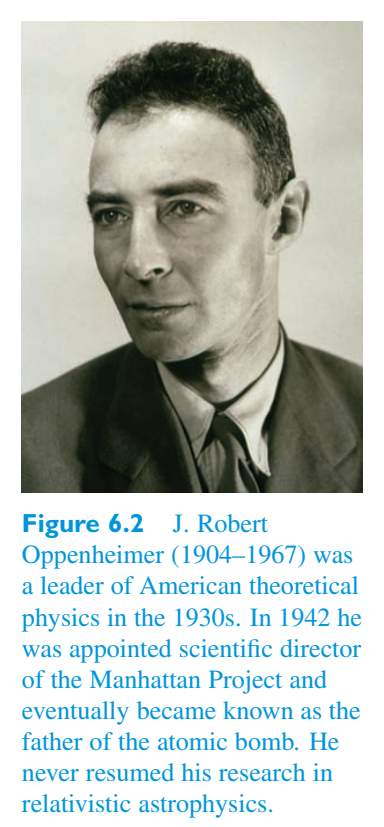
- ●●
What general relativistic effect should be expected to cause a distant observer’s view of a collapsing star’s surface to be reddened compared with the view of an observer falling with the surface?与随表面坠落的观察者的视野相比,什么样的广义相对论效应会导致远处观察者看到的正在塌缩的恒星表面变红?
❍ Gravitational redshift will cause radiation emitted from the surface to have a smaller frequency (i.e. to be redder) according to a distant observer than according to an observer moving with the surface.❍ 引力红移将导致从表面发射的辐射在远处的观察者看来比在随表面移动的观察者看来具有更小的频率(即更红)。
The 1940s and 1950s are generally regarded as a sterile time for general relativity. There were real achievements but the field faced difficult problems that some thought to be insurmountable, and there was a lack of relevant experimental information to check or challenge the existing theory. However, things began to change at the end of that period, setting the scene for a renaissance of general relativity in the 1960s that would revitalize the field and bring black holes into prominence.20世纪40年代和1950年代通常被认为是广义相对论的贫瘠时期。虽然取得了实际成果,但该领域面临着一些人认为无法克服的难题,并且缺乏相关的实验信息来检验或挑战现有的理论。然而,在那段时期末,情况开始发生变化,为 20 世纪 60 年代广义相对论的复兴奠定了基础,这将重振该领域并使黑洞成为人们关注的焦点。
In 1958, rediscovering a coordinate system first used by Eddington in the 1920s, the American mathematical physicist David Finkelstein (1929–) showed how the Schwarzschild metric could be partly freed of its coordinate singularity and used to discuss separately the inward and outward motion of photons in the neighbourhood of the Schwarzschild radius. Then, in 1960, Martin Kruskal (1925–2006) in the USA and George Szekeres (1911–2005) in Australia independently found a coordinate system that allowed a unified description of the Schwarzschild solution, free of coordinate singularities. Soon after came the first observations of peculiar star-like astronomical bodies that would later be given the name quasars (short for quasi-stellar objects) and would eventually be recognized as the highly active nuclei of remote but luminous galaxies. So prodigious was the outpouring of energy from quasars that many felt that they had to involve some kind of energy-generating mechanism that was quite different from the nuclear reactions that powered normal stars.1958 年,美国数学物理学家戴维·芬克尔斯坦 (David Finkelstein,1929-) 重新发现了爱丁顿在 20 年代首次使用的坐标系,并展示了如何将史瓦西度规部分地摆脱其坐标奇点,并用于分别讨论史瓦西半径附近光子的向内和向外运动。然后,在 1960 年,美国的 Martin Kruskal(1925-2006)和澳大利亚的 George Szekeres(1911-2005)独立地找到了一个坐标系,可以统一描述史瓦西解,没有坐标奇点。不久之后,人们首次观测到了奇特的类星体天体,这些天体后来被命名为类星体(准恒星天体的缩写),并最终被认为是遥远但明亮的星系的高度活跃的核。类星体释放出的能量如此巨大,以至于许多人认为它们必须涉及某种能量产生机制,这种机制与为普通恒星提供动力的核反应完全不同。
Over a relatively short period during the 1960s, the ideas of gravitational collapse and black holes underwent a rapid development that took them from the fringes to the centre of astrophysical thinking. In 1963 New Zealander Roy Kerr (1934–) discovered the solution of the vacuum field equations that would later be used to describe realistic rotating black holes, just as the Schwarzschild metric would be used for non-rotating black holes. Roger Penrose (1931–) introduced the first of a number of singularity theorems showing that gravitational singularities were an inevitable consequence of complete gravitational collapse. A number of investigators suggested that the release of gravitational potential energy by matter (about 3 solar masses per year) falling into a compact object with a mass of about 10 8 solar masses could account for the energy emitted by quasars. It was in this fervid atmosphere that John Archibald Wheeler (Figure 6.3), who had been urging the field forward since the late 1950s, introduced the term ‘black hole’ in 1967. In 1969 the term ‘event horizon’ (which had been introduced some years earlier in a different context) was applied to the surface surrounding a gravitationally collapsed object that separated the events that might be seen by a distant observer from those that were forever cut off from such an observer. The black hole with its central singularity and surrounding event horizon had arrived.在 20 世纪 60 年代相对较短的时间内,引力塌缩和黑洞的思想经历了快速发展,使它们从天体物理学思想的边缘走向了中心。 1963 年,新西兰人 Roy 克尔(1934-)发现了真空场方程的解,该方程后来被用于描述现实的旋转黑洞,就像史瓦西度规用于非旋转黑洞一样。罗杰·彭罗斯(Roger Penrose,1931-)提出了许多奇点定理中的第一个,表明引力奇点是完全引力崩溃的不可避免的结果。许多研究人员认为,物质(每年约 3 个太阳质量)落入质量约为 10 8 个太阳质量的致密天体时释放的引力势能可以解释类星体释放的能量。正是在这种热烈的气氛中,自 20 世纪 50 年代末以来一直推动该领域向前发展的约翰·阿奇博尔德·惠勒 (John Archibald Wheeler)(图 6.3)于 1967 年引入了“黑洞”一词。1969年,“事件视界”一词(几年前在不同的背景下引入)被应用于引力塌陷物体周围的表面,它将远处观察者可能看到的事件与永远与观察者隔绝的事件分开。具有中心奇点和周围事件视界的黑洞已经到来。
Of course, many subsequent developments followed, but to the extent that we discuss them at all we shall treat them as they arise in the discussion below. Let us end this section with some words from Wheeler.当然,随后出现了许多后续发展,但就我们讨论它们而言,我们将按照下面讨论中出现的方式对待它们。让我们用惠勒的一些话来结束本节。
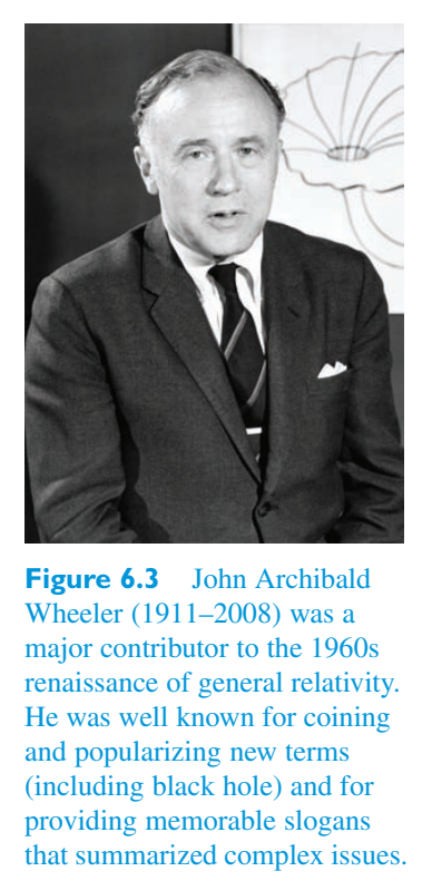
The black hole epitomizes the revolution wrought by general relativity. It pushes to an extreme — and therefore tests to the limit — the features of general relativity (the dynamics of curved spacetime) that set it apart from special relativity (the physics of static, ‘flat’ spacetime) and the earlier mechanics of Newton.黑洞是广义相对论带来的革命的缩影。它将广义相对论(弯曲时空的动力学)的特征推向了极限,从而将其与狭义相对论(静态、“平坦”时空的物理学)和早期牛顿力学区分开来。
J.A. Wheeler (1998) Geons, Black Holes & Quantum Foam, NortonJ.A.惠勒 (1998) 几何子、黑洞和量子泡沫,诺顿
6.1.3 The classification of black holes6.1.3 黑洞的分类
The basis of the most common classification scheme for black holes is John Wheeler’s pronouncement that ‘a black hole has no hair’. What Wheeler meant by this was that a black hole has very few independent, externally measurable properties; namely, its mass, its angular momentum and its electric charge. All black holes must have mass, so there are only four basic types of black hole. An essentially unique metric is now known for each of those types, including the Schwarzschild metric for those with no charge and no angular momentum. The full four-fold classification scheme looks like this.黑洞最常见的分类方案的基础是约翰·惠勒的声明“黑洞没有毛发”。惠勒的意思是黑洞几乎没有独立的、外部可测量的特性;即它的质量、角动量和电荷。所有黑洞都必须有质量,因此黑洞只有四种基本类型。现在,每种类型都有一个本质上独特的度规标准,包括用于不带电荷和角动量的史瓦西度规标准。完整的四重分类方案如下所示。
PROPERTIES METRIC Mass only Schwarzschild Mass and angular momentum Kerr Reissner–Nordstro¨m Mass and electric charge Mass, angular momentum and electric charge Kerr–Newman属性度规仅质量史瓦西质量和角动量克尔 Reissner–Nordstrom 质量和电荷质量、角动量和电荷克尔–Newman
It is expected that real black holes will have angular momentum, but may well not be charged since atoms tend to be neutral. Because of this we shall discuss rotating and non-rotating black holes but we shall mainly ignore charged black holes.预计真正的黑洞将具有角动量,但很可能不带电,因为原子往往是中性的。因此,我们将讨论旋转和非旋转黑洞,但我们将主要忽略带电黑洞。
Another widely used classification scheme for black holes is perhaps more relevant to astrophysics. It is based on the mass of the black hole. The mass limits of the various classes are not precisely defined and several authors have proposed new classes. Here is a version of the scheme.另一种广泛使用的黑洞分类方案可能与天体物理学更相关。它是基于黑洞的质量。各种类别的质量限制没有精确定义,一些作者提出了新的类别。这是该方案的一个版本。
CLASS MASS RANGE 0 to 0.1 M) Mini black holes类质量范围 0 至 0.1 M) 迷你黑洞
0.1 to 300 M)0.1至300M)
Stellar mass black holes Intermediate mass black holes 300 to 10 5 M) 10 5 to \(10^{10}\) M) Supermassive black holes恒星质量黑洞中等质量黑洞 300 至 10 5 M) 10 5 至 \(10^{10}\) M) 超大质量黑洞
Many authors who discuss mini black holes suppose them to have masses very much less than the mass of the Sun — less, say, than the mass of the Moon — and some have even discussed subdivisions such as micro black holes or nano black holes. However, given the rather imprecise nature of this classification scheme, we shall simply make do with the broad category of mini black holes.许多讨论微型黑洞的作者认为它们的质量远小于太阳的质量——比方说,小于月球的质量——有些甚至讨论了诸如微型黑洞或纳米黑洞之类的细分。然而,考虑到这种分类方案相当不精确,我们将简单地使用迷你黑洞这一广泛的类别。
- ● If the accretion of matter by a black hole, at the rate● 如果黑洞吸积物质的速率为
of a few solar masses per year, explains the luminosity of quasars, what kind of black hole would you expect to be responsible?每年几个太阳质量,解释类星体的光度,你认为哪种黑洞负责?
❍ Real black holes are expected to be rotating and uncharged, so a Kerr black hole is most likely. Also, if the suggested rate of fuelling is to account for the observed energy release from quasars, the black hole would need to have a mass of order 10 8 solar masses, so it would be in the supermassive class.❍ 真正的黑洞预计会旋转且不带电,因此克尔黑洞最有可能。此外,如果建议的燃料供给速率是为了考虑到观测到的类星体的能量释放,那么黑洞的质量需要达到 10 8 个太阳质量,因此它将属于超大质量级别。
To summarize, here are the main results of this section.总而言之,以下是本节的主要结果。
Black holes黑洞
A black hole is a region of spacetime that matter and radiation may enter but from which they may not escape. The region is bounded by an event horizon that separates events that can be seen by an external observer from those that cannot be seen. At the heart of a black hole is a singularity that may arise from the complete gravitational collapse of a star or some other body. The limiting masses of white dwarfs and neutron stars indicate the possibility of gravitational collapse, but the consequences were first investigated in detail by Oppenheimer and his collaborators. The term black hole was introduced by Wheeler in the 1960s when there was a renaissance in the study of general relativity, partly inspired by the need to account for the prodigious energy output from quasars. Black holes are commonly classified according to their mass or according to the solution of the vacuum field equations that describes them. The only independent externally measurable properties of a black hole are its mass, charge and angular momentum.黑洞是物质和辐射可以进入但无法逃脱的时空区域。该区域以事件视界为界,将外部观察者可以看到的事件与无法看到的事件分开。黑洞的中心是一个奇点,它可能是由于恒星或其他天体的完全引力塌缩而产生的。白矮星和中子星的极限质量表明引力坍缩的可能性,但奥本海默和他的合作者首先详细研究了其后果。黑洞这个术语是由惠勒在 20 世纪 60 年代提出的,当时广义相对论研究正在复兴,部分原因是需要考虑类星体的巨大能量输出。黑洞通常根据其质量或根据描述它们的真空场方程的解进行分类。黑洞唯一可独立外部测量的属性是其质量、电荷和角动量。
6.2 Non-rotating black holes6.2 非旋转黑洞
As pointed out in Chapter 5, Birkhoff’s theorem establishes the uniqueness of the Schwarzschild solution in describing the spacetime external to a source that has spherically symmetric effects. So, whether discussing the spherically symmetric collapse of a non-rotating star or the spherically symmetric black hole that might be expected to result from such a collapse, the Schwarzschild solution will play a central role.正如第五章所指出的,伯克霍夫定理确立了史瓦西解在描述具有球对称效应的源外部时空方面的唯一性。因此,无论是讨论非旋转恒星的球对称坍缩,还是讨论这种坍缩可能导致的球对称黑洞,史瓦西解都将发挥核心作用。
In this section we shall return to a number of the topics that were introduced in Chapter 5 but our concern will be mainly with events at or around the Schwarzschild radius, which will turn out to be the location of the event horizon of a non-rotating black hole. Since it is described by the Schwarzschild metric, we shall sometimes refer to a non-rotating black hole as a Schwarzschild black hole. We shall see some further consequences of the lack of immediate metrical significance of the Schwarzschild coordinates, ct and r, and give further thought to the implications of geodesic motion, including the motion of photons, which we largely ignored earlier.在本节中,我们将回顾第 5 章中介绍的一些主题,但我们主要关注史瓦西半径或周围的事件,这将是非旋转黑洞的事件视界的位置。由于它是通过史瓦西度规来描述的,因此我们有时将非旋转黑洞称为史瓦西黑洞。我们将看到史瓦西坐标 ct 和 r 缺乏直接度规意义的一些进一步后果,并进一步思考测地线运动的含义,包括我们之前很大程度上忽略的光子运动。
To start with we shall follow in the footsteps of Oppenheimer and his collaborators by considering the proper time taken for a freely falling observer to reach the central singularity of a Schwarzschild spacetime.首先,我们将追随奥本海默和他的合作者的脚步,考虑自由落体观察者到达史瓦西时空中心奇点所需的固有时间。
6.2.1 Falling into a non-rotating black hole6.2.1 落入不旋转黑洞
In Worked Example 5.1 we showed that in Schwarzschild spacetime the radial motion of a freely falling body with non-zero mass agreed with Newtonian expectations provided that (i) the speed of the body is much less than c, and (ii) the gravitational field is weak (i.e. there is negligible spacetime curvature). Let us now consider the behaviour of a radially falling body that violates these conditions by passing though the event horizon and travelling on towards r = 0. As in the worked example, our starting point is the radial motion equation but we shall use \(R_S\) = 2 GM/\(c^2\) to write it in the form在工作示例 5.1 中,我们表明,在史瓦西时空中,具有非零质量的自由落体物体的径向运动符合牛顿期望,前提是(i)物体的速度远小于 c,并且(ii)引力场很弱(即时空曲率可以忽略不计)。现在让我们考虑一下径向落体的行为,它通过事件视界并朝 r = 0 方向移动,从而违反了这些条件。如在工作示例中,我们的起点是径向运动方程,但我们将使用 \(R_S\) = 2 GM/\(c^2\) 将其写成以下形式
The constant E represents the energy, the value of which is determined by the initial conditions. On this occasion we shall suppose that the fall starts from rest at some large value of r which we shall denote \(r_0\), so d r/d \(\tau\) = 0 when r = \(r_0\) and常数E代表能量,其值由初始条件决定。在这种情况下,我们假设下降从静止开始,在 r 的某个大值处,我们将其表示为 \(r_0\),因此当 r = \(r_0\) 时,d r/d \(\tau\) = 0 且
It follows that由此可见
Taking the negative square root to describe inward motion (r decreasing as取负平方根来描述向内运动(r 减小为
Taking the reciprocal, we can rewrite this as取倒数,我们可以将其重写为
Integrating both sides with respect to r, from the starting point \(r_0\) to some general point \(r'\), gives the proper duration of the fall as对 r 两侧进行积分,从起点 \(r_0\) 到某个一般点 \(r'\),给出正确的下落持续时间:
The integral can be found in tables of standard integrals or (with appropriate caution) using an algebraic computing package. It turns out that积分可以在标准积分表中找到,或者(适当谨慎)使用代数计算包。事实证明
Substituting the appropriate limits we see that代入适当的限制我们可以看到
For the case we are interested in, when \(r_0 \ll r\), expanding the functions on the right in power series leads to the approximation对于我们感兴趣的情况,当 \(r_0 \ll r\) 时,展开幂级数右侧的函数会得到近似值
If we allow the general point \(r'\) to approach the central singularity by considering the limit \(r'\) → 0, we find that the total proper time for the fall is finite and has value如果我们通过考虑极限 \(r'\) → 0 让一般点 \(r'\) 逼近中心奇点,我们发现下落的总本征时间是有限的并且具有值
Another significant result that also follows from Equation另一个重要结果也可以从方程得出
6.7 is the proper time6.7是适当的时间
required to fall from \(r_0\) to the event horizon at \(r'\) = \(R_S\). The result is需要从 \(r_0\) 落到 \(r'\) = \(R_S\) 处的事件视界。结果是
The difference between these last two results is the proper time required for the freely falling body to travel from the horizon to the singularity, which is just最后两个结果之间的差异是自由落体从视界行进到奇点所需的固有时间,即
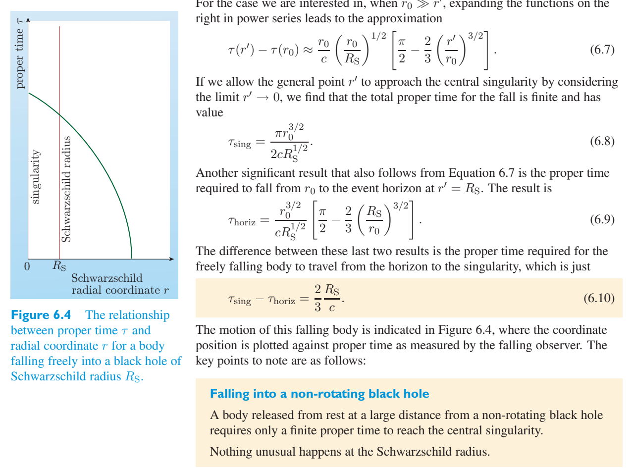
The motion of this falling body is indicated in Figure 6.4, where the coordinate position is plotted against proper time as measured by the falling observer. The key points to note are as follows:该下落物体的运动如图 6.4 所示,其中坐标位置是根据下落观察者测量的原时时间绘制的。需要注意的要点如下:
Falling into a non-rotating black hole掉入不旋转的黑洞
A body released from rest at a large distance from a non-rotating black hole requires only a finite proper time to reach the central singularity.距离非旋转黑洞很远的地方从静止状态释放出来的物体只需要有限的固有时间即可到达中心奇点。
Nothing unusual happens at the Schwarzschild radius.在史瓦西半径范围内没有发生任何异常情况。
Exercise 6.1 (a) What is the proper time required练习 6.1 (a) 所需的固有时间是多少
for a falling body to travel from the Schwarzschild radius to the singularity of a black hole with 3 times the mass of the Sun?一个下落的物体从史瓦西半径行进到质量是太阳三倍的黑洞奇点?
(b) What is the corresponding proper travel time for a fall from the horizon to the singularity of a supermassive black hole of mass \(10^9M_\odot\)?(b) 质量为 \(10^9M_\odot\) 的超大质量黑洞从地平线坠落到奇点的相应本征旅行时间是多少?
6.2.2 Observing a fall from far away6.2.2 远处观察跌倒
For a distant stationary observer, at rest far from the origin, there is no essential difference between the proper time that would be measured on a clock and the coordinate time t. To avoid confusion with the proper time \(\tau\) recorded by the freely falling observer, we shall always use t when discussing observations made by the distant observer.对于一个远离原点的静止观察者来说,在时钟上测量的本征时间和坐标时间 t 之间没有本质区别。为了避免与自由落体观察者记录的本征时间 \(\tau\) 混淆,在讨论远处观察者的观察时,我们将始终使用 t。
The first thing that we need to know is how long it takes for a light signal emitted by the freely falling body to reach the distant observer. To be specific we shall suppose that the distant observer is located along the same radial line that the falling body is moving along, simply further out. That means we only have to consider photons that travel radially from the falling body to the distant observer. For events along the path of such a photon, d \(\theta\) = d \(\phi\) = 0. We already know that the spacetime separation (d s) 2 of events on a photon’s world-line is zero, so it follows from the Schwarzschild metric that for two events on the world-line of a photon travelling radially outwards,我们首先需要知道的是,自由落体发出的光信号需要多长时间才能到达远处的观察者。具体来说,我们假设远处的观察者位于落体移动的同一径向线上,只是更远一些。这意味着我们只需要考虑从下落物体径向传播到远处观察者的光子。对于沿着这样一个光子路径的事件,d \(\theta\) = d \(\phi\) = 0。我们已经知道,光子世界线上事件的时空间隔 (d s) 2 为零,因此根据史瓦西度规,对于径向向外传播的光子世界线上的两个事件,
Rearranging and taking square roots, we see that for radially moving photons,重新排列并求平方根,我们看到对于径向移动的光子,
where the − sign applies to photons travelling radially inwards (d r deceasing) while the + sign applies to the outward-moving photons that interest us. This relation holds true for neighbouring events all along the world-line of the photon, so for a photon emitted from the falling body at t 1 and r 1 that is observed by the distant observer at \(t_{2}\) and \(r^2\), the total journey time is given by其中 - 号适用于径向向内传播的光子(d r 递减),而 + 号适用于我们感兴趣的向外移动的光子。这种关系对于沿着光子世界线的邻近事件都成立,因此对于在 t 1 和 r 1 处从落体发射的光子,并由远处观察者在 \(t_{2}\) 和 \(r^2\) 处观察到,总行程时间由下式给出
Evaluating the integral gives计算积分给出
There are three important points to note about Equation 6.14.关于公式 6.14,需要注意三个要点。
First, the coordinate time interval is not simply (\(r^2\) − r 1)/c. This, of course, is because the coordinates lack immediate metrical significance, especially close to the Schwarzschild radius.首先,坐标时间间隔不是简单的(\(r^2\) − r 1)/c。当然,这是因为坐标缺乏直接的度规意义,特别是在史瓦西半径附近。
Second, the journey time is always greater than (\(r^2\) − r 1)/c due to the additional logarithmic term. As the point of emission, r 1, gets closer and closer to the Schwarzschild radius, this logarithmic term becomes larger and larger. Indeed, as r 1 → \(R_S\) so \(t_{2}\) − t 1 → ∞. So, as seen by the distant observer, the falling body will never quite reach the event horizon.其次,由于附加的对数项,行程时间始终大于 (\(r^2\) − r 1)/c。随着发射点 r 1 越来越接近史瓦西半径,这个对数项变得越来越大。事实上,由于 r 1 → \(R_S\) 所以 \(t_{2}\) − t 1 → ∞。因此,正如远处的观察者所看到的那样,下落的物体永远不会完全到达事件视界。
Third, the difference in coordinate time between emission and observation depends only on the coordinate positions of the emitter and observer. As long as the positions remain fixed, signals will always take the same amount of coordinate time to travel from r 1 to \(r^2\), and signals emitted with coordinate time intervals \(\Delta w\)ill arrive with coordinate time intervals \(\Delta t\). This justifies an assertion that we made in Chapter 5, concerning a stationary emitter and a stationary observer, when we said that the coordinate time interval between the emissions of two successive signals was the same as the coordinate time interval between their receptions.第三,发射和观察之间的坐标时间差仅取决于发射器和观察者的坐标位置。只要位置保持固定,信号将始终花费相同的坐标时间从 r 1 传播到 \(r^2\),并且以坐标时间间隔 \(\Delta w\) 发出的信号将以坐标时间间隔 \(\Delta t\) 到达。这证明了我们在第五章中关于静止发射器和静止观察者的断言,当时我们说两个连续信号发射之间的坐标时间间隔与它们接收之间的坐标时间间隔相同。
We can get a more detailed picture of what the distant observer will see if we determine the position of the freely falling body as a function of coordinate position d r to time t. To do this we need to relate the differences in coordinate differences in coordinate time d t for events on the world-line of the falling body.如果我们将自由落体的位置确定为坐标位置 d r 与时间 t 的函数,我们就可以更详细地了解远处观察者将看到的情况。为此,我们需要关联落体世界线上事件的坐标时间 d t 的坐标差异。
d r and d t. Why can’td r 和 d t。为什么不能
- ● Equation 6.12 already provides a relationship between● 公式 6.12 已经提供了以下关系:
we just use that?我们只是用那个?
❍ That equation only applies to events on the world-line of a photon. It was deduced from the metric using the condition (d s) 2 = 0. We need a condition that applies to events on the world-line of a freely falling body with non-zero mass.❍ 该方程仅适用于光子世界线上的事件。它是使用条件 (d s) 2 = 0 从度规中推导出来的。我们需要一个适用于具有非零质量的自由落体物体的世界线上的事件的条件。
We considered the motion of a freely falling body in Chapter 5, where one of the results that we introduced (Equation 5.28 after substituting \(R_S\) for \(2GM/c^2\)) was我们在第 5 章考虑了自由落体的运动,其中我们引入的一个结果(方程 5.28,把 \(2GM/c^2\) 记作 \(R_S\) 后)是
Now we already know, from Equation 6.4, that for a body starting its fall from rest at a large distance \(r_0\) from the origin, \(E/mc^2=(1-R_S/r_0)^{1/2}\). Substituting this into Equation 6.15 and rearranging, we see that for events on the world-line of the freely falling body,现在由方程 6.4 可知,对于从距离原点很远的 \(r_0\) 处由静止开始下落的物体,\(E/mc^2=(1-R_S/r_0)^{1/2}\)。将其代入方程 6.15 并整理,可得自由落体世界线上的事件满足
We also considered a freely falling body earlier in this chapter, eventually arriving at我们在本章前面也考虑了自由落体,最终得到
Multiplying these last two results together gives the desired relation between \(dt\) and \(dr\) for events along the world-line of a freely falling body with non-zero mass:将最后两个结果相乘,就得到具有非零质量的自由落体物体世界线上事件所需的 \(dt\) 与 \(dr\) 之间的关系:
Analysing this general relationship is possible but complicated, so we shall use the fact that we are mainly interested in effects at or near the event horizon, where r is small compared with \(r_0\), to justify the simplification that分析这种一般关系是可能的,但很复杂,因此我们将利用我们主要感兴趣的是事件视界处或事件视界附近的效应(其中 r 与 \(r_0\) 相比较小)这一事实来证明以下简化的合理性:
Integrating both sides with respect to r, from a point at radial coordinate r ∗ that is much larger than \(R_S\) but much less than \(r_0\), to some general point \(r'\), gives对 r 两侧进行积分,从远大于 \(R_S\) 但远小于 \(r_0\) 的径向坐标 r * 处的点到某个通用点 \(r'\),给出
The integral can be found in tables or by using an algebraic computing package:积分可以在表格中或通过使用代数计算包找到:
Substituting the limits, we get the final answer代入极限,得到最终答案
This relationship is illustrated in Figure 6.5, which also includes a line representing the curve that we obtained earlier when plotting the radial coordinate against proper time. Remembering that we approximated the equation of motion before performing the integral, the constant has been chosen to ensure that the two curves match at r = r ∗, where intervals of coordinate time t and proper time \(\tau\) are essentially the same. As r becomes smaller, the two curves separate, with t becoming infinite as r → \(R_S\). So we again see that according to a distant observer it takes an infinite time for a body falling into a black hole to reach the event horizon. Note that this infinity concerns the coordinate time that the falling body requires to reach the horizon; it is quite distinct from the time required for a light signal from the body to reach a distant observer.这种关系如图 6.5 所示,其中还包括一条代表我们之前在绘制径向坐标与原时坐标时获得的曲线的线。请记住,我们在执行积分之前近似了运动方程,选择常数是为了确保两条曲线在 r = r ∗ 处匹配,其中坐标时间 t 和本征时间 \(\tau\) 的间隔基本相同。随着 r 变小,两条曲线分开,t 变得无穷大,因为 r → \(R_S\)。因此,我们再次看到,根据遥远的观察者的说法,落入黑洞的物体需要无限的时间才能到达事件视界。请注意,这个无穷大涉及下落物体到达地平线所需的坐标时间;它与身体发出的光信号到达远处观察者所需的时间截然不同。
As noted earlier, light emitted from a falling body approaching a black hole will exhibit an increasing gravitational redshift according to a distant observer. The formula for gravitational redshift from a stationary source was given in Chapter 5:如前所述,根据远处的观察者的说法,接近黑洞的落体发出的光将表现出不断增加的引力红移。第 5 章给出了固定源的引力红移公式:
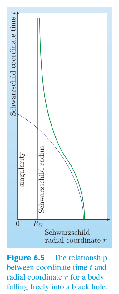
Using the general relationship c = f \(\lambda\), we can express the redshift in terms of wavelength as使用一般关系 c = f \(\lambda\),我们可以将波长的红移表示为
The formulae predict that the observed redshift will become greater and greater as the point of emission approaches the event horizon. Indeed, as r → \(R_S\), \(\lambda\) ∞ → ∞. For this reason the event horizon is often described as a surface of infinite redshift.这些公式预测,随着发射点接近事件视界,观测到的红移将变得越来越大。事实上,当 r → \(R_S\),\(\lambda\) ∞ → ∞ 时。因此,事件视界通常被描述为无限红移的表面。
Actually, the redshift seen by a distant observer will increase even more rapidly than the formula indicates since our earlier result applied to a stationary source while the falling body that we are now considering will be moving away from the distant observer. This motion will cause a Doppler shift that will further increase the observed redshift, though the event horizon will remain a surface of infinite redshift.实际上,远处观察者看到的红移会比公式所示的增加得更快,因为我们之前的结果适用于固定源,而我们现在考虑的落体将远离远处观察者。这种运动将引起多普勒频移,从而进一步增加观测到的红移,尽管事件视界仍将是无限红移的表面。
Another effect follows from those that we have already mentioned. Suppose that the falling body is emitting light with a constant luminosity L 0 according to an observer falling with it. The increasing redshift (which reduces the energy per photon) and the extended time of emission and travel (which reduces the rate at which photons are received) will all tend to decrease the luminosity of the source as seen by a distant observer. During the early part of the fall, the distant observer will see the source becoming dimmer due to its increasing distance from the observer, but the additional dimming due to general relativistic effects will become more pronounced as the falling body is seen to approach the event horizon. Quantitative studies show that if the light is treated as continuous classical radiation (i.e. ignoring the fact that it is actually emitted as photons), then in the final stages of the observed fall, the dimming becomes exponential, measured luminosity halving on a timescale of order \(R_S\)/c, so另一个效果来自我们已经提到过的效果。假设根据与它一起下落的观察者,下落体发出具有恒定光度L 0 的光。红移的增加(减少每个光子的能量)以及发射和传播时间的延长(减少光子接收的速率)都会降低远处观察者所看到的光源的光度。在坠落的早期阶段,远处的观察者会看到光源由于距观察者的距离不断增加而变得越来越暗,但是当坠落体接近事件视界时,由于广义相对论效应而导致的额外变暗将变得更加明显。定量研究表明,如果将光视为连续的经典辐射(即忽略它实际上以光子形式发射的事实),然后在观察到的下降的最后阶段,变暗呈指数变化,测量到的光度在 \(R_S\)/c 量级的时间尺度上减半,所以
where a is a constant of order 1. This is such a rapid dimming that, far from the falling body being visible for all eternity, such a body would actually become unobservably dim rather quickly once it gets close to the event horizon.其中 a 是 1 阶常数。这种变暗速度如此之快,以至于坠落的物体远非永远可见,一旦接近事件视界,这样的物体实际上会很快变得难以观察到的暗淡。
All this talk of bodies falling into a black hole may sound rather fanciful, but remember that the body concerned might, in principle, be part of the surface of a star undergoing gravitational collapse. In this way the ideas that we have been discussing can form the basis for observational predictions concerning the behaviour of a star as it undergoes gravitational collapse and contracts within its own Schwarzschild radius. The interested reader can pursue this topic elsewhere but we should note again the key points to emerge from our discussion.所有这些关于物体落入黑洞的讨论可能听起来相当异想天开,但请记住,原则上,相关物体可能是正在经历引力坍缩的恒星表面的一部分。通过这种方式,我们一直在讨论的想法可以构成对恒星在其史瓦西半径内经历引力坍缩和收缩时的行为的观测预测的基础。有兴趣的读者可以在其他地方继续讨论这个话题,但我们应该再次注意我们讨论中出现的要点。
Observing a body fall into a non-rotating black观察物体落入不旋转的黑色区域
hole洞
A body falling into a black hole takes an infinite amount of coordinate time to reach the event horizon. Light signals emitted from the object also take an increasing amount of (coordinate) time to reach a distant observer. These effects will reduce the rate at which photons from the falling body reach the distant observer. Signals from the falling body are also redshifted according to the distant observer, with the horizon representing a surface of infinite redshift. This reduces the energy per photon received by the distant observer. The combination of all these effects will cause an in-falling body of constant proper luminosity to dim rapidly as it approaches the horizon.落入黑洞的物体需要无限的坐标时间才能到达事件视界。从物体发出的光信号也需要越来越长的(坐标)时间才能到达远处的观察者。这些效应将降低落体光子到达远处观察者的速率。根据远处的观察者的说法,来自坠落物体的信号也会发生红移,地平线代表无限红移的表面。这减少了远处观察者接收到的每个光子的能量。所有这些效应的结合将导致具有恒定适当光度的下落天体在接近地平线时迅速变暗。
Exercise 6.2 A light pulse is emitted in the outward练习 6.2 向外发射光脉冲
direction from a source just exterior to the event horizon of a non-rotating black hole. Write down an expression for the radial speed of light according to a stationary local observer and according to a stationary observer at infinity, and show that both are equal to c.来自非旋转黑洞事件视界外部源的方向。写出根据静止本地观察者和根据无穷远静止观察者的光径向速度的表达式,并证明两者都等于 c。
Exercise 6.3 According to a local observer, stationary练习 6.3 根据当地观察者的说法,静止
just outside the event horizon of a non-rotating black hole, what is the speed of a freely falling body, travelling radially inwards, as it nears the event horizon, given that the body was released from rest at a great distance from the black hole?就在非旋转黑洞的事件视界之外,考虑到该物体在距离黑洞很远的地方从静止状态释放出来,当它接近事件视界时,自由落体径向向内运动的速度是多少?
Exercise 6.4 Imagine watching an astronaut falling练习 6.4 想象一下看着一名宇航员坠落
freely into a non-rotating black hole, waving goodbye as he or she approaches the event horizon. What might a distant observer expect to see?自由地进入一个不旋转的黑洞,当他或她接近事件视界时挥手告别。远处的观察者可能期望看到什么?
6.2.3 Tidal effects near a non-rotating black hole6.2.3 非旋转黑洞附近的潮汐效应
It’s natural to expect that anyone falling into a stationary black hole will be crushed to death in its central singularity. However, this expectation overlooks tidal effects.很自然地,任何落入静止黑洞的人都会在其中心奇点处被压死。然而,这种预期忽略了潮汐效应。
Tides are a familiar phenomenon on the Earth. They arise primarily from variations in the gravitational field due to the Moon and the Sun across the diameter of the Earth. The basis of the Newtonian explanation of tides is illustrated for the case of lunar tides in Figure 6.6.潮汐是地球上常见的现象。它们主要是由于月球和太阳在地球直径上引起的引力场的变化而产生的。牛顿潮汐解释的基础如图 6.6 中的月球潮汐情况所示。
If the oceans are represented by a uniformly deep layer of water, then at any point on that water surface there is a lunar tidal field given by the (vector) difference between the local value of the gravitational field due to the Moon and its value at the centre of the Earth. The effect of this tidal field is to redistribute the oceans in such a way that the water surface forms an equipotential surface of the combined Earth–Moon gravitational field.如果海洋由均匀的深层水代表,那么在该水面上的任何点都存在月球潮汐场,该月球潮汐场由月球引力场的局部值与其在地球中心的引力场值之间的(矢量)差给出。该潮汐场的作用是重新分布海洋,使水面形成地月引力场的等位面。
If we consider the Earth and the Moon in isolation, the key points to note are as follows.如果我们孤立地考虑地球和月球,需要注意的要点如下。
- • If the Earth and the Moon were point particles in an isolated system bound by如果地球和月球是一个孤立系统中的点粒子,
gravity, each particle would be in free fall about the common centre of mass of the system.在引力作用下,每个粒子都会围绕系统的共同质心自由落体。
- • As they are extended bodies with finite diameters, the individual centres of由于它们是具有有限直径的延伸体,因此各个中心
mass of the Earth and the Moon are in free fall about their common centre of mass (which is actually some way beneath the Earth’s surface), but the same is not true of all other points in those bodies.地球和月球的质量围绕它们的共同质心(实际上位于地球表面以下的某个位置)做自由落体运动,但这些天体中的所有其他点并非如此。
- • The Moon’s gravitational field is stronger at point A in Figure 6.6 than at月球引力场在图 6.6 中的 A 点处比在
point C, causing material at point A to experience a tidal force towards the Moon and therefore away from the centre of the Earth.C 点,导致 A 点的物质受到朝向月球的潮汐力,从而远离地球中心。
- • The Moon’s gravitational field is weaker at point D in Figure 6.6 than at月球引力场在图 6.6 中的 D 点处比在
point C, causing material at point D to experience a tidal force away from the Moon, but this is also away from the centre of the Earth.C点,导致D点的物质受到远离月球的潮汐力,但这也远离地球的中心。
- • The Moon’s gravitational field at point B is inclined at an angle to the月球在 B 点的引力场与月球引力场成一定角度。
gravitational field at point C in Figure 6.6, causing material at point B to experience a tidal force almost perpendicular to the direction towards the Moon and directed towards the centre of the Earth.图 6.6 中 C 点的引力场,导致 B 点的物质受到几乎垂直于月球方向并指向地球中心的潮汐力。
- • In the case of the solid Earth, the response to the tidal• 对于固体地球,对潮汐的响应
field and the forces that it produces is small. The electrical forces between atoms in a solid are so strong that only a small (but measurable) distortion of the solid Earth is sufficient to produce forces that counterbalance the tidal forces. The same is not true of the oceans. The forces between atoms in a liquid are much weaker than those that act within a solid. In response to the tidal field the oceans rise or fall until the additional weight of the water column at any point counterbalances the tidal force. Put differently, the oceans redistribute themselves in such a way that they form a surface of uniform gravitational potential in the combined gravitational field of the Earth and the Moon. Hence the observed tidal bulges.场及其产生的力很小。固体中原子之间的电力非常强大,以至于固体地球仅发生很小的(但可测量的)变形就足以产生抵消潮汐力的力。海洋则不然。液体中原子之间的作用力比固体中原子之间的作用力弱得多。为了响应潮汐场,海洋上升或下降,直到任何点上水柱的附加重量抵消了潮汐力。换句话说,海洋以这样的方式重新分布自身,从而在地球和月球的联合引力场中形成均匀引力势的表面。因此观察到的潮汐隆起。
Note that this Newtonian argument involves free fall and variations in the gravitational field across the diameter of the Earth. (Also note that it has nothing to do with ‘centrifugal forces’ as some sources incorrectly claim.) In reality there are additional effects that arise from the rotation of the Earth and the particular form of ocean basins and coastlines, but these are specific to the Earth, so we shall not pursue them here.请注意,这个牛顿论证涉及自由落体和地球直径上引力场的变化。 (另请注意,它与某些来源错误地声称的“离心力”无关。)实际上,地球自转以及海洋盆地和海岸线的特殊形式会产生额外的影响,但这些是地球特有的,因此我们不会在这里追究它们。
A body falling freely towards a black hole will also be subject to tidal effects. In general relativity it would be inappropriate to describe these effects in terms of the different gravitational forces on the body, since there are no gravitational forces in general relativity. Rather, we should use the language of spacetime curvature and geodesic motion, though we should be able to recover the idea of tidal forces from the relativistic description in the appropriate Newtonian limit.自由落向黑洞的物体也会受到潮汐效应的影响。在广义相对论中,用物体上的不同引力来描述这些效应是不合适的,因为广义相对论中不存在引力。相反,我们应该使用时空曲率和测地运动的语言,尽管我们应该能够在适当的牛顿极限下从相对论描述中恢复潮汐力的概念。
The usual starting point for a relativistic account of tidal effects is the concept of geodesic deviation, which will now be described. Consider a region of spacetime, and suppose that C and D are two parameterized curves passing though that region. More specifically, suppose that C and D are neighbouring geodesics, so each curve is the possible world-line of a particle passing though the region. The functions [x \(\mu\) C (\(\lambda\))], geodesic C can be represented by a set of four coordinate where \(\lambda\) is an affine parameter, and we shall suppose that its neighbouring geodesic D is affinely parameterized in such a way that it can be described by a similar set of coordinate functions [x \(\mu\) (\(\lambda\))]. Because C and D are neighbouring geodesics parameterized in similar ways, we can suppose that corresponding to each value of \(\lambda\) is a unique pair of points, one on C and the other on D, separated by a four-dimensional separation [ξ \(\mu\) (\(\lambda\))], where潮汐效应相对论解释的通常起点是测地偏差的概念,现在将对其进行描述。考虑一个时空区域,并假设 C 和 D 是穿过该区域的两条参数化曲线。更具体地说,假设 C 和 D 是相邻的测地线,因此每条曲线都是穿过该区域的粒子的可能世界线。函数 [x \(\mu\) C (\(\lambda\))],测地线 C 可以由一组四个坐标表示,其中 \(\lambda\) 是仿射参数,并且我们假设其相邻测地线 D 被仿射参数化,使得它可以由一组类似的坐标函数 [x \(\mu\) (\(\lambda\))] 描述。因为 C 和 D 是以类似方式参数化的相邻测地线,所以我们可以假设与 \(\lambda\) 的每个值对应的是一对唯一的点,一个在 C 上,另一个在 D 上,由四维间隔分开 [xi \(\mu\) (\(\lambda\))],其中
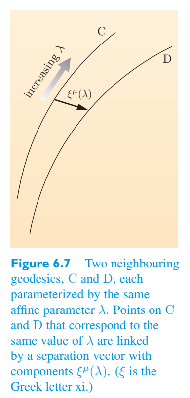
[ξ \(\mu\) (\(\lambda\))] is illustrated in This arrangement of geodesics and their separation vector Figure 6.7.[xi \(\mu\) (\(\lambda\))] 在测地线的这种排列及其分离向量图 6.7 中进行了说明。
In the absence of gravity, in a region where the Riemann curvature is zero and spacetime is flat, it is easy to imagine that the geodesics will be straight lines that particles move along at constant speed. In such circumstances, the separation vector [ξ \(\mu\)] will be constant. However, in the presence of gravity, spacetime will be curved, the Riemann curvature will be non-zero, particles on neighbouring geodesics can have relative accelerations, and the behaviour of the separation vector might be complicated. In fact, a detailed analysis shows that the changes in the separation vector are described by the following equation of geodesic deviation.在没有引力的情况下,在黎曼曲率为零且时空平坦的区域中,很容易想象测地线将是粒子以恒定速度移动的直线。在这种情况下,分离向量[xi \(\mu\)]将是恒定的。然而,在存在引力的情况下,时空将会弯曲,黎曼曲率将不为零,相邻测地线上的粒子可能具有相对加速度,并且分离矢量的行为可能会很复杂。事实上,详细分析表明,分离矢量的变化是用下面的测地偏差方程来描述的。
Equation of geodesic deviation测地偏差方程
This relationship holds at all points along the geodesic C, and the expression D 2 ξ \(\mu\)/D \((\lambda)^2\) represents the second-order derivative along the curve C of the separation vector component ξ \(\mu\). This kind of derivative is similar in some respects to the covariant derivative that was introduced in Chapter 4. In the case of the covariant derivative we noted that when differentiating tensor components such as T \(\mu\) \(\nu\) with respect to coordinates x \(\rho\), the partial derivatives ∂T \(\mu\) \(\nu\)/∂x \(\rho\) do not generally transform as the components of a tensor, but we were able to construct a related quantity that we denoted ∇ \(\rho\) T \(\mu\) \(\nu\), that was a kind of derivative and produced a result that was a tensor of higher rank. In the present case, when considering changes in ξ \(\mu\) as we move from event to event along the geodesic C, we need to differentiate with respect to the affine parameter \(\lambda\) in such a way that the rank 1 tensor nature of ξ \(\mu\) will not change. This is what is provided by the derivative along the curve, which is defined by这种关系在测地线 C 上的所有点上都成立,并且表达式 D 2 xi \(\mu\)/D \((\lambda)^2\) 表示分离矢量分量 ψ \(\mu\) 沿曲线 C 的二阶导数。这种导数在某些方面与第 4 章中介绍的协变导数类似。在协变导数的情况下,我们注意到,当对坐标 x \(\rho\) 微分张量分量(例如 T \(\mu\) \(\nu\))时,偏导数 ∂T \(\mu\) \(\nu\)/∂x \(\nu\)/∂x \(\rho\) 通常不会转换为张量的分量,但我们能够构造一个我们表示的相关量∇ \(\rho\) T \(\mu\) \(\nu\),这是一种导数,产生的结果是更高阶的张量。在本例中,当我们沿着测地线 C 从一个事件移动到另一个事件时,当考虑 xi \(\mu\) 的变化时,我们需要对仿射参数 \(\lambda\) 进行微分,使得 xi \(\mu\) 的 1 阶张量性质不会改变。这就是沿曲线的导数所提供的,其定义为
Taking a second derivative results in a complicated expression that simplifies to Equation 6.23.求二阶导数会得到一个复杂的表达式,可简化为公式 6.23。
In the Newtonian limit, when speeds are low and gravitational fields are weak, the equation of geodesic deviation will provide information about the relative acceleration of freely falling particles as they move along neighbouring geodesics — which is exactly the kind of information needed to work out Newtonian tidal fields. However, the equation of geodesic deviation is not restricted to the Newtonian limit. As a covariant tensor relationship, it provides the essential generalization of Newtonian tidal fields that makes it possible to describe tidal effects throughout curved Schwarzschild spacetime, apart from the central singularity where tidal effects become infinite.在牛顿极限下,当速度较低且引力场较弱时,测地偏差方程将提供有关自由落体粒子沿相邻测地线移动时的相对加速度的信息,这正是计算牛顿潮汐场所需的信息。然而,测地偏差方程并不局限于牛顿极限。作为一种协变张量关系,它提供了牛顿潮汐场的基本概括,使得可以描述整个弯曲的史瓦西时空中的潮汐效应,除了潮汐效应变得无限的中心奇点之外。
In the case of an astronaut falling feet first towards a non-rotating black hole, the result of geodesic deviation is disastrous. While the astronaut’s centre of mass falls into the central singularity in the proper time calculated earlier, the astronaut’s head and feet will arrive at significantly different times! During the inward fall, geodesic deviation stretches the astronaut in the radial direction and causes compression in the transverse directions. This process is usually referred to as spaghettification and is illustrated schematically in Figure 6.8.如果宇航员双脚先落向不旋转的黑洞,测地线偏差的结果将是灾难性的。虽然宇航员的质心在之前计算出的固有时间落入中心奇点,但宇航员的头部和脚部到达的时间却明显不同!在向内坠落过程中,测地偏差使宇航员在径向方向上拉伸,并在横向方向上造成压缩。该过程通常称为意大利面条化,如图 6.8 所示。
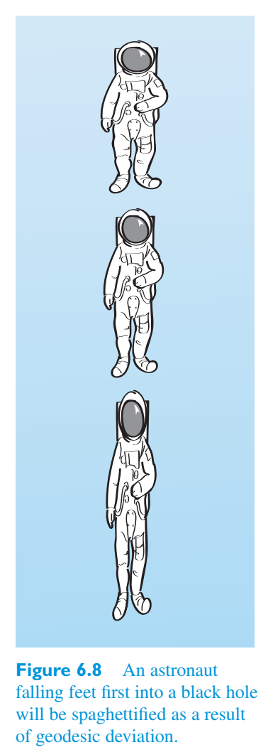
Spaghettification will generally kill an in-falling astronaut before the astronaut reaches the central singularity. Indeed, in the case of a stellar mass black hole, death from spaghettification will usually occur well before the astronaut crosses the event horizon. We can estimate where the effect becomes significant by working in the Newtonian approximation. The magnitude of the Newtonian gravitational field (force per unit test mass) at a distance r from a body of mass M is在宇航员到达中心奇点之前,面条化通常会导致坠落的宇航员死亡。事实上,在恒星质量黑洞的情况下,因意大利面条化而死亡通常会在宇航员穿过事件视界之前发生。我们可以通过牛顿近似来估计影响在哪里变得显着。距质量体 M 距离 r 处的牛顿引力场(每单位测试质量的力)大小为
If δr represents a small change in the radial coordinate, we can use Taylor’s theorem to determine the corresponding change in the field. Working to first order,如果δr代表径向坐标的微小变化,我们可以利用泰勒定理来确定场的相应变化。按第一顺序工作,
where δf is a measure of the tidal force per unit mass acting along an object of d r | = 2 GM/\(r^3\) provides dimension δr. The magnitude of the field gradient | d f/a useful measure of tidal lethality. This quantity is very large near the event horizon of a stellar mass black hole, partly due to the large mass of the black hole, but more particularly because r is already small near the Schwarzschild radius. A human body is unlikely to survive a gradient of order 10 4 \(\mathrm{s^{-2}}\). This is the kind of field gradient that would be encountered at about 1000 km from a 40 solar mass black hole, far beyond the event horizon, which would be at about 120 km from the centre. In the case of a supermassive black hole with a mass of 10 7 solar masses, the event horizon would be at \(3\times10^{7}\) km and the field gradient at the horizon would be only about 10 − 4 \(\mathrm{s^{-2}}\), too small for a falling astronaut to notice. The falling astronaut who passed through the event horizon would not be able to escape, but would still have a long way to fall before the tidal effects became lethal.其中 δf 是沿 d r | 物体作用的单位质量潮汐力的度规。 = 2 GM/\(r^3\) 提供尺寸 δr。场梯度的大小| d f/潮汐致死率的有用衡量标准。这个量在恒星质量黑洞的事件视界附近非常大,部分原因是黑洞的质量很大,但更具体的是因为 r 在史瓦西半径附近已经很小。人体不可能承受 10 4 \(\mathrm{s^{-2}}\) 量级的梯度。这种场梯度会在距 40 个太阳质量的黑洞约 1000 公里处遇到,远远超出事件视界(距中心约 120 公里)。在质量为 10 7 个太阳质量的超大质量黑洞的情况下,事件视界将位于 \(3\times10^{7}\) km,视界处的场梯度仅为约 10 − 4 \(\mathrm{s^{-2}}\),对于坠落的宇航员来说太小而无法注意到。穿过事件视界的坠落宇航员将无法逃脱,但在潮汐效应变得致命之前,还有很长的路要走。
6.2.4 The deflection of light near a non-rotating6.2.4 光在非旋转物体附近的偏转
black hole黑洞
When discussing motion in Schwarzschild spacetime in Chapter 5, we started our discussion of the geodesics in a general way that included massless particles such as photons, as well as particles with mass. However, we soon focused on the case of massive particles and essentially ignored the motion of photons. In this chapter we have already used the metric to discuss the radial motion of photons, but we have still not paid any attention to the non-radial motion of photons. We shall now remedy that omission.当第五章讨论史瓦西时空中的运动时,我们开始以一般的方式讨论测地线,其中包括光子等无质量粒子以及有质量的粒子。然而,我们很快就把注意力集中在大质量粒子的情况上,而基本上忽略了光子的运动。在本章中我们已经使用度规来讨论光子的径向运动,但我们仍然没有关注光子的非径向运动。我们现在将弥补这一遗漏。
Figure 6.9 shows the trajectories of photons (or any other massless particles) moving in a plane that also contains the central singularity of a non-rotating black hole of Schwarzschild radius \(R_S\). The trajectories are initially parallel but each can be identified by its impact parameter, that is, the perpendicular (coordinate) distance b from the singularity to the initial direction of motion of the photon. Values of the impact parameter are shown on the vertical axis in the figure, expressed as multiples of the Schwarzschild radius.图 6.9 显示了光子(或任何其他无质量粒子)在平面中移动的轨迹,该平面还包含史瓦西半径为 \(R_S\) 的非旋转黑洞的中心奇点。这些轨迹最初是平行的,但每个轨迹都可以通过其影响参数来识别,即从奇点到光子初始运动方向的垂直(坐标)距离 b。冲击参数的值显示在图中的垂直轴上,表示为史瓦西半径的倍数。
As you can see, photons with b = 3 \(R_S\) or b = 4 \(R_S\) are strongly deflected, though they are not drawn into the black hole. This is an example of the phenomenon of light deflection, mentioned in Chapter 4, that Einstein was able to predict on the basis of the principle of equivalence. The effect becomes weaker as the impact parameter increases but remains detectable even for large multiples of the impact parameter. We shall have more to say about this phenomenon in the next chapter when we discuss tests of general relativity.正如您所看到的,b = 3 \(R_S\) 或 b = 4 \(R_S\) 的光子被强烈偏转,尽管它们没有被吸入黑洞。这是第四章中提到的光偏转现象的一个例子,爱因斯坦能够根据等效原理进行预测。随着影响参数的增加,效果会变弱,但即使对于影响参数的大倍数,效果仍然可以检测到。当我们讨论广义相对论的检验时,我们将在下一章中更多地讨论这一现象。
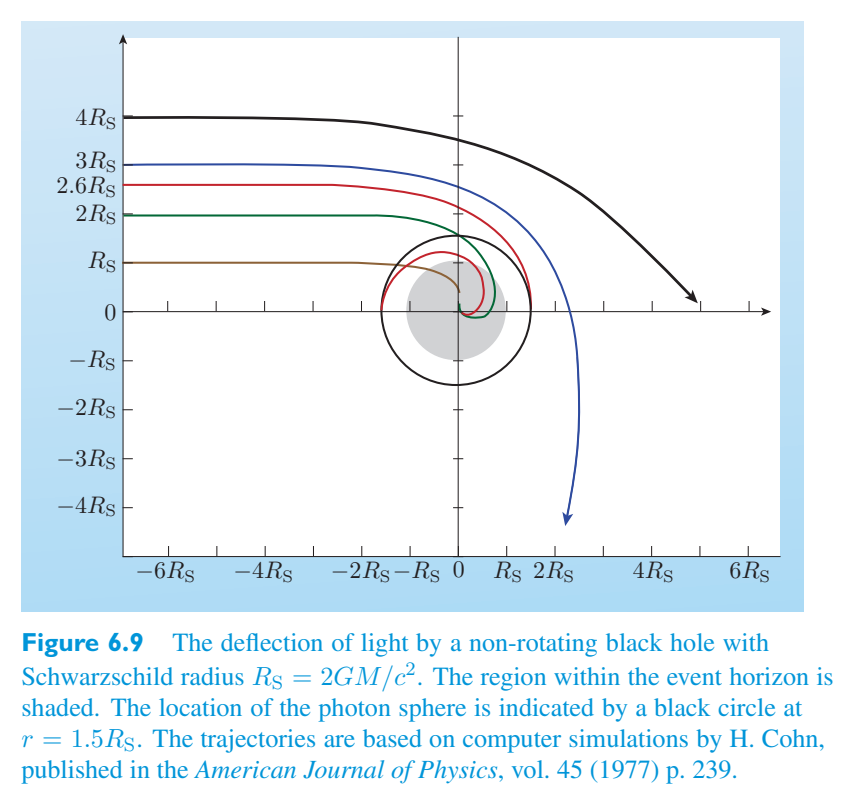
6.2.5 The event horizon and beyond6.2.5 事件视界及其以外
We saw earlier that, as measured by a distant observer, a body falling into a non-rotating black hole takes an infinite amount of coordinate time to reach the event horizon. However, we also saw that such a body, as observed by a freely falling observer travelling with it, requires only a finite proper time to pass through the event horizon and continue on to the central singularity. Interestingly, there are values of the Schwarzschild coordinates that correspond to all events on the inward journey, apart from the coordinate singularity at the Schwarzschild radius. The full journey is shown in Figure 6.10.我们之前看到,根据远处观察者的测量,落入非旋转黑洞的物体需要无限长的坐标时间才能到达事件视界。然而,我们也看到,这样一个物体,正如与它一起旅行的自由落体观察者所观察到的那样,只需要有限的固有时间就可以穿过事件视界并继续到达中心奇点。有趣的是,除了史瓦西半径处的坐标奇点之外,史瓦西坐标的值与向内旅程中的所有事件相对应。完整行程如图6.10所示。
As you can see, the extra part of the pathway (shown in orange) from the horizon to the central singularity starts as t → ∞ and leads back in coordinate time to some earlier finite value! It’s tempting to interpret this as a sign that the in-falling observer is travelling backwards in time. However, no such fanciful interpretation is needed. It is true that the value of t is decreasing, but you have already learned that in general relativity coordinates lack immediate metrical significance. The decreasing value of Schwarzschild coordinate time t for an in-falling observer inside the event horizon simply shows that the Schwarzschild coordinates are especially poorly suited to the task of describing the last stages of the fall.正如您所看到的,从地平线到中心奇点的路径的额外部分(以橙色显示)从 t → ∞ 开始,并在坐标时间内返回到某个较早的有限值!人们很容易将此解释为坠落观察者正在时光倒流的迹象。然而,不需要这种奇特的解释。确实,t 的值正在减小,但您已经了解到,在广义相对论中,坐标缺乏直接的度规意义。对于事件视界内的坠落观察者来说,史瓦西坐标时间 t 的减小值仅仅表明史瓦西坐标特别不适合描述坠落最后阶段的任务。
More evidence of the inappropriateness of Schwarzschild coordinates can be obtained by using them to describe the lightcones along the path of an in-falling observer. It was shown in Chapter 1 that lightcones provide a valuable tool for investigating the causal structure of spacetime. In that earlier application we were concerned with the geometrically flat Minkowski spacetime of special relativity, where lightcones could be extended to infinity without any impediment. In contrast, in general relativity, spacetime is generally curved, so lightcones cannot be indefinitely extended. Nonetheless, observers using locally inertial frames (such as freely falling observers) will find that special relativity holds true Schwarzschild radial locally, so any such observer can use lightcones to explore the local structure of spacetime.通过使用史瓦西坐标来描述沿着坠落观察者的路径的光锥,可以获得更多证明史瓦西坐标不合适的证据。第一章表明,光锥为研究时空因果结构提供了一个有价值的工具。在早期的应用中,我们关注的是狭义相对论中几何平坦的闵可夫斯基时空,其中光锥可以毫无障碍地延伸到无穷大。相反,在广义相对论中,时空通常是弯曲的,因此光锥不能无限延伸。尽管如此,使用局部惯性系的观察者(例如自由落体观察者)会发现狭义相对论在局部保持真实的史瓦西径向,因此任何这样的观察者都可以使用光锥来探索时空的局部结构。
The local lightcones in Schwarzschild spacetime can be identified from a spacetime diagram showing incoming and outgoing null geodesics (i.e. possible photon world-lines). Just such a diagram is shown in Figure史瓦西时空中的局部光锥可以从显示传入和传出零测地线(即可能的光子世界线)的时空图中识别出来。就是这么一个图如图所示
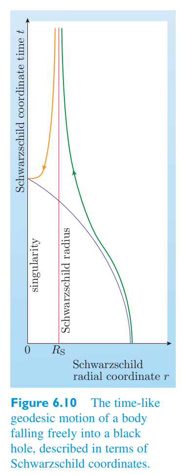
6.11. The figure uses这一关系在测地线 C 上的所有点都成立,表达式 D 2 ξ \(\mu\)/D \((\lambda)^2\) 表示分离矢量分量 ξ \(\mu\) 沿曲线 C 的二阶导数。这种导数在某些方面类似于第 4 章介绍的协变导数。对于协变导数,我们曾注意到,当相对于坐标 x \(\rho\) 对张量分量如 T \(\mu\) \(\nu\) 求导时,偏导数 ∂T \(\mu\) \(\nu\)/∂x \(\rho\) 通常不会像张量分量那样变换;但我们可以构造一个相关量,记为 ∇ \(\rho\) T \(\mu\) \(\nu\),它是一种导数,并产生更高阶张量的结果。在现在的情形中,当我们沿测地线 C 从一个事件移动到另一个事件并考虑 ξ \(\mu\) 的变化时,需要以一种不改变 ξ \(\mu\) 的一阶张量性质的方式,对仿射参数 \(\lambda\) 求导。这正是沿曲线的导数所提供的,它定义为
Schwarzschild coordinates, the axes being ct and r. The curves are described by Equation 6.12, which was obtained directly from the Schwarzschild metric for the that (d s) 2 = 0 for case of radial motion together with the additional requirement the quantity d(ct)/d r, photons. Rearranging that equation slightly, to emphasize which describes the gradient of the lightcone’s edge, we get史瓦西坐标,轴为 ct 和 r。这些曲线由方程 6.12 描述,该方程是直接从史瓦西度规获得的,对于径向运动的情况,(d s) 2 = 0 以及附加要求量 d(ct)/d r,光子。稍微重新排列该方程,以强调它描述了光锥边缘的梯度,我们得到
Note that far from the horizon, as r → ∞, this equation implies that d(ct)/d r = ± 1, so that lightcones take the form that they would have in special relativity. However, when approaching the horizon from outside, d(ct)/d r → ±∞, causing the lightcones to become very narrow. Just inside the horizon something even more remarkable occurs. The lightcones suddenly become very broad again, and their time-like regions become horizontal, so that the only possible directions of radial motion are towards the singularity. You saw an example of this in Figure 6.10, where the last part of the time-like orange curve was almost horizontal, but Figure 6.11 shows that this is a general phenomenon. The tipping of the lightcones (see Figure请注意,远离地平线,当 r → ∞ 时,该方程意味着 d(ct)/d r = ± 1,因此光锥采用狭义相对论中的形式。然而,当从外部接近地平线时,d(ct)/d r → ±∞,导致光锥变得非常狭窄。就在地平线内,发生了更引人注目的事情。光锥突然再次变得非常宽,它们的类时间区域变得水平,因此径向运动唯一可能的方向是朝向奇点。您在图 6.10 中看到了一个这样的示例,其中类似时间的橙色曲线的最后部分几乎是水平的,但图 6.11 表明这是一种普遍现象。光锥的倾斜(见图
6.12) makes a certain kind6.12) 制作某种类型
of sense since it indicates the inevitability of encountering the singularity once the event horizon has been passed. However, the abrupt switch in direction and the sudden broadening of the lightcones looks very odd and is another sign of inappropriateness of the Schwarzschild coordinates in this region.这是有意义的,因为它表明一旦经过事件视界,就不可避免地会遇到奇点。然而,方向的突然转变和光锥的突然变宽看起来非常奇怪,并且是史瓦西坐标在该区域不合适的另一个迹象。
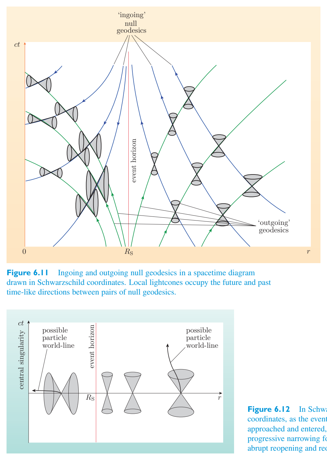
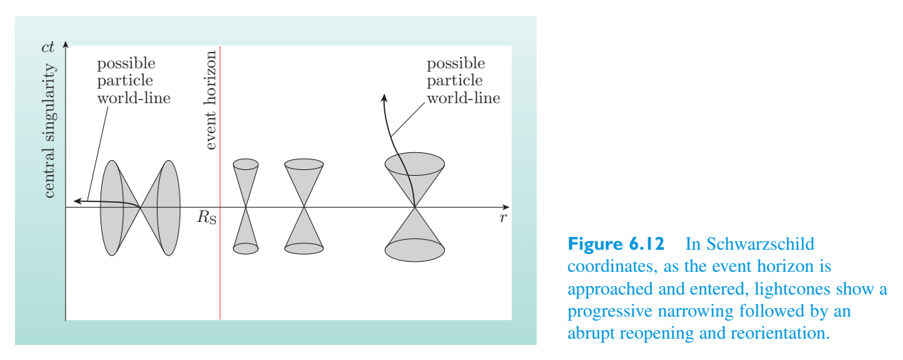
Many of the coordinate-related problems associated with non-rotating black holes can be removed by changing the coordinates used to describe them. The necessary transformation was introduced in the late 1950s by Finkelstein, though he was rediscovering coordinates that had been introduced for a different purpose by Eddington in 1924.许多与非旋转黑洞相关的坐标相关问题可以通过改变用于描述它们的坐标来消除。芬克尔斯坦 (Finkelstein) 在 20 世纪 50 年代末引入了必要的变换,尽管他正在重新发现爱丁顿 (Eddington) 于 1924 年出于不同目的引入的坐标。
In what are known as advanced Eddington–Finkelstein coordinates, a new coordinate \(t'\) is related to the Schwarzschild t and r coordinates by the equation在所谓的高级爱丁顿-芬克尔斯坦坐标中,新坐标 \(t'\) 通过以下方程与史瓦西 t 和 r 坐标相关
With this modified time coordinate, the line element of Schwarzschild spacetime can be written as通过这个修改后的时间坐标,史瓦西时空的线元可以写为
which is non-singular at r = \(R_S\). In these coordinates ingoing null geodesics are represented by straight lines while outgoing photons are curves. (Of course, those within the event horizon don’t actually go outwards, they just arrive at the central singularity at a later value of \(t'\).) The relevant spacetime diagram for advanced Eddington–Finkelstein coordinates is shown in Figure 6.13, and the corresponding sequence of lightcones is shown in Figure它在 r = \(R_S\) 处是非奇异的。在这些坐标中,传入的零测地线由直线表示,而传出的光子则由曲线表示。(当然,事件视界内的那些实际上并没有向外出去,它们只是在 \(t'\) 的较晚值处到达中心奇点。)高级爱丁顿-芬克尔斯坦坐标的相关时空图如图 6.13 所示,相应的光锥序列如图 6.13 所示。
6.14.6.14。
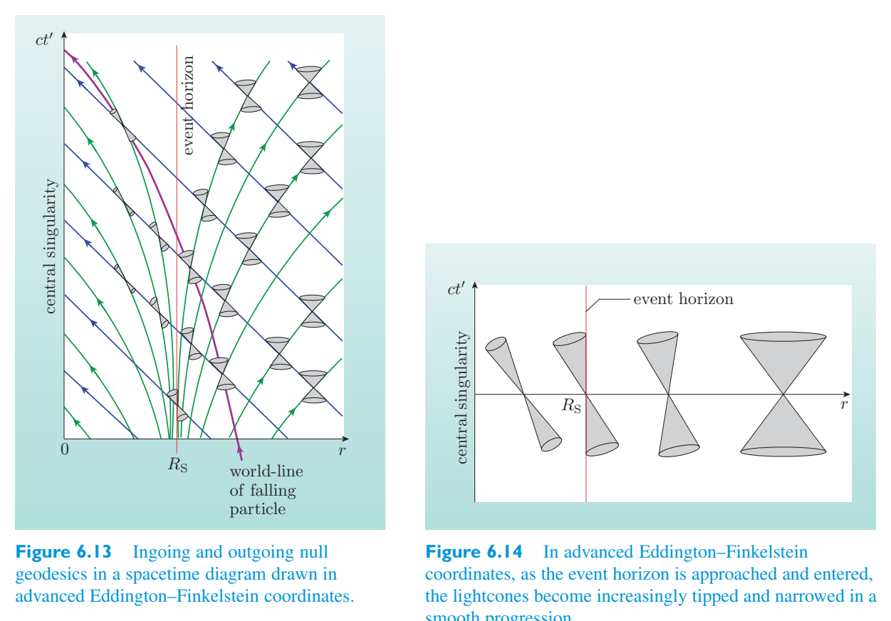
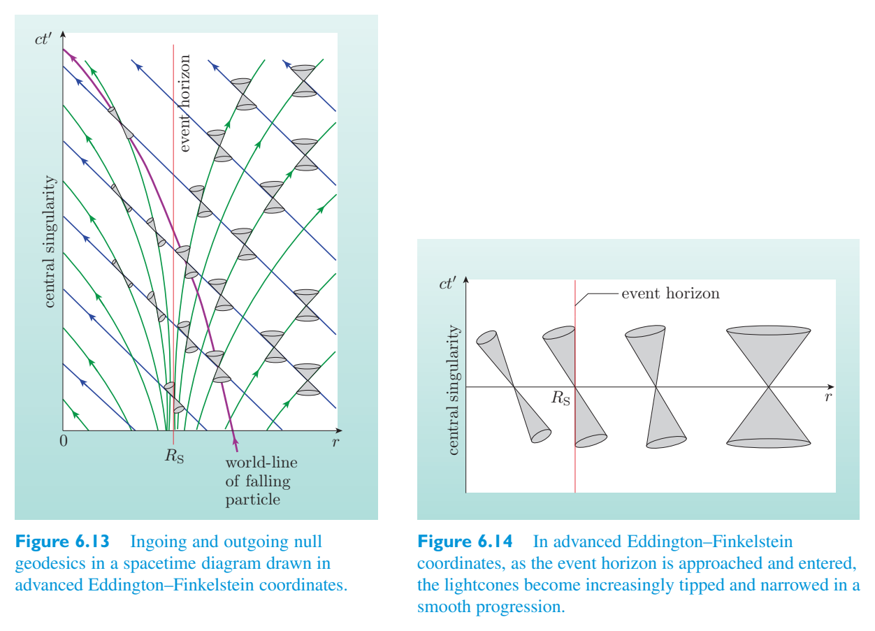
geodesics in a spacetime diagram drawn in advanced Eddington–Finkelstein coordinates.以高级爱丁顿-芬克尔斯坦坐标绘制的时空图中的测地线。
The ‘opening-up’ of Schwarzschild spacetime that advanced Eddington–Finkelstein coordinates permit is the start of a new chapter in the investigation of black holes, not the end of one. In Schwarzschild coordinates there is a symmetry between ingoing and outgoing null geodesics, yet in advanced Eddington–Finkelstein coordinates an asymmetry is introduced: the ingoing null geodesics are straight, the outgoing ones are not. This suggests the existence of another coordinate system that would in some sense reverse the asymmetry. Such a coordinate system does exist, and the two types of Eddington–Finkelstein coordinates together were a step towards a further development. In 1960, Martin Kruskal introduced a single set of coordinates that were non-singular everywhere outside the physical singularity. In these coordinates it is natural to extend the domain covered by the usual Schwarzschild solution. Indeed, in this context the Schwarzschild solution is seen to be just one half of a broader domain referred to as its maximal analytic extension (see Figure 6.15). The existence of this mathematically extended domain has given rise to many speculations about ‘other universes’, spacetime ‘wormholes’, and ‘white holes’ from which matter and radiation might be expelled with the same kind of inevitability that they are drawn into a black hole. We shall not discuss these aspects of the Schwarzschild solution, though you may like to follow them up in other sources. However, it is appropriate to end with two final points. The first is to note that some physicists take the view that the extended domain is physically inaccessible and therefore of little interest and no scientific relevance. The second is to note that in a field as complicated as general relativity it has often taken a long time for the physical significance of mathematical results to be fully appreciated; humility in the face of complexity is sometimes an appropriate response.先进的爱丁顿-芬克尔斯坦坐标允许的史瓦西时空的“开放”是黑洞研究新篇章的开始,而不是结束。在史瓦西坐标中,传入和传出零测地线之间存在对称性,但在高级爱丁顿-芬克尔斯坦坐标中引入了不对称性:传入零测地线是直的,传出零测地线不是直的。这表明存在另一个坐标系,该坐标系在某种意义上可以逆转不对称性。这样的坐标系确实存在,两种类型的爱丁顿-芬克尔斯坦坐标结合在一起是进一步发展的一步。 1960 年,马丁·克鲁斯卡尔 (Martin Kruskal) 引入了一组坐标,该坐标在物理奇点之外的任何地方都是非奇异的。在这些坐标中,很自然地扩展通常的史瓦西解所覆盖的域。事实上,在这种情况下,史瓦西解被视为只是更广泛的域的一半,称为其最大分析扩展(见图 6.15)。这个数学扩展域的存在引发了许多关于“其他宇宙”、时空“虫洞”和“白洞”的猜测,物质和辐射可能会像被吸入黑洞一样不可避免地被排出。我们不会讨论史瓦西解的这些方面,尽管您可能想在其他来源中跟进它们。然而,最后两点是适当的。首先要注意的是,一些物理学家认为扩展域在物理上是不可访问的,因此没有什么意义,也没有科学意义。其次要注意的是,在像广义相对论这样复杂的领域中,通常需要很长时间才能充分理解数学结果的物理意义;面对复杂性,谦虚有时是适当的反应。
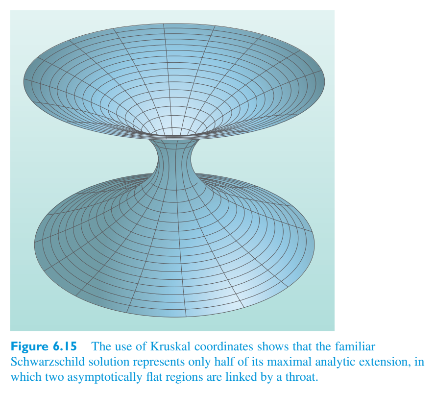
Lightcones, spacetime diagrams and event horizons光锥、时空图和视界
Lightcones and spacetime diagrams are valuable tools for investigating local spacetime structure in general relativity, but the behaviour of lightcones will depend on the particular coordinates being used. In Schwarzschild coordinates lightcones show abrupt changes at the Schwarzschild radius, which is the location of a coordinate singularity. Advanced Eddington–Finkelstein coordinates remove the coordinate singularity and produce lightcones that change in a regular way, tipping and narrowing as they approach the Schwarzschild radius. The behaviour of the lightcones at and within the Schwarzschild radius indicates the inevitability of encountering the central singularity, though more powerful methods must be used to prove that inevitability.光锥和时空图是研究广义相对论中局部时空结构的宝贵工具,但光锥的行为将取决于所使用的特定坐标。在史瓦西坐标中,光锥在史瓦西半径(坐标奇点的位置)处显示出突变。高级爱丁顿-芬克尔斯坦坐标消除了坐标奇点并产生以规则方式变化的光锥,当它们接近史瓦西半径时倾斜和变窄。史瓦西半径处和之内的光锥的行为表明遇到中心奇点的必然性,尽管必须使用更强大的方法来证明这种必然性。
Exercise 6.5 When working in advanced Eddington–Finkelstein练习 6.5 在高级 Eddington-Finkelstein 中工作时
coordinates, which feature(s) of the lightcones suggest the impossibility of escaping from within the event horizon of a non-rotating black hole?坐标,光锥的哪些特征表明不可能从非旋转黑洞的事件视界内逃逸?
Exercise 6.6 Using (a) Schwarzschild coordinates练习 6.6 使用 (a) 史瓦西坐标
and (b) advanced Eddington–Finkelstein coordinates, sketch spacetime diagrams showing the time-like geodesic of a radially in-falling body. In each case add to the geodesic future lightcones representing the development of flashes of light emitted by that body during its fall. Include the region inside the event horizon as well as the region outside the horizon.(b) 先进的爱丁顿-芬克尔斯坦坐标,草图时空图显示了径向下落物体的类时间测地线。在每种情况下,添加代表该物体在坠落过程中发出的闪光的发展的测地线未来光锥。包括事件视界内的区域以及视界外的区域。
6.3 Rotating black holes6.3 旋转黑洞
Real astrophysical systems, such as stars and galaxies, generally possess angular momentum. A body that undergoes a gravitational collapse is expected to retain a good deal of the angular momentum that it has immediately prior to the collapse. In addition, as you will see later, a black hole may acquire angular momentum from in-falling bodies. For all of these reasons, real black holes, if they exist, are expected to rotate. This section is devoted to rotating black holes.真实的天体物理系统,例如恒星和星系,通常具有角动量。经历引力塌缩的物体预计会保留塌缩前的大量角动量。此外,正如您稍后将看到的,黑洞可能会从下落的物体中获得角动量。由于所有这些原因,真正的黑洞如果存在的话,预计会旋转。本节专门讨论旋转黑洞。
6.3.1 The Kerr solution and rotating black6.3.1 克尔解和旋转黑
holes洞
Our starting point for the description of a non-rotating black hole was the Schwarzschild solution, which describes the spacetime outside a spherically symmetric body. The solution has the properties of being stationary (so that the metric coefficients are independent of t), spherically symmetric, asymptotically flat, singular and (loosely speaking) unique.我们描述非旋转黑洞的起点是史瓦西解,它描述了球对称体外部的时空。该解具有平稳(以便度规系数独立于 t)、球对称、渐近平坦、奇异和(松散地说)唯一的属性。
We cannot expect the Schwarzschild solution to describe a rotating black hole because the black hole’s angular momentum will pick out some particular direction in space and that will destroy the spherical symmetry. We might, though, expect there to be some sort of analogue of the Schwarzschild solution with the properties of being stationary, axially symmetric (i.e. having the invariance of a cylinder), asymptotically flat and singular. We might also hope that some kind of extension or generalization of Birkhoff’s theorem will again establish the essentially unique character of the solution. Just such a solution was discovered by Roy Kerr in 1963, though it took some time for its uniqueness to be established.我们不能指望史瓦西解来描述旋转的黑洞,因为黑洞的角动量会在空间中找出一些特定的方向,从而破坏球对称性。不过,我们可能期望存在某种史瓦西解的类似物,具有静止、轴对称(即具有圆柱体的不变性)、渐近平坦和奇异的性质。我们可能还希望伯克霍夫定理的某种扩展或概括将再次确立该解决方案本质上独特的特征。 Roy 克尔于 1963 年发现了这样的解决方案,尽管它的独特性花了一些时间才被确立。
The line element of the Kerr solution can be written as follows.克尔解的线元可以写成如下。
Kerr line element克尔线元
This looks (and is) rather complicated, but there are some key points to note.这看起来(而且确实)相当复杂,但有一些关键点需要注意。
- • The Kerr metric depends on just two parameters, \(R_S\) = 2 GM/\(c^2\) and克尔度规仅取决于两个参数,RS = 2 GM/\(c^2\) 和
a = J/(M c), which in turn depend on the mass M and angular momentum magnitude J. The metric describes a black hole only when a ≤ \(R_S\)/2, i.e. when J ≤ GM 2/c, and the important limiting case when a = \(R_S\)/2 is said to describe an extreme Kerr black hole.a = J/(M c),这又取决于质量 M 和角动量大小 J。只有当 a ≤ RS/2(即 J ≤ GM 2/c)时,该度规才描述黑洞,并且当 a = RS/2 时的重要极限情况被认为描述了极端克尔黑洞。
- • The coordinates used to describe the metric, ct, r, \(\theta\), \(\phi\), are called用于描述度规 ct、r、\(\theta\)、\(\phi\) 的坐标称为
Boyer–Lindquist coordinates. \(\phi\) is a standard spherical coordinate, but \(\theta\) and r are not. They are related to standard Cartesian coordinates x and y by博耶-林德奎斯特坐标。 \(\phi\) 是标准球坐标,但 \(\theta\) 和 r 不是。它们与标准笛卡尔坐标 x 和 y 的关系为
r is still a kind of radial coordinate, but increasing values of r do not correspond to spheres of increasing proper circumference, nor does r = 0 identify a unique point. At a fixed value of t, a surface of constant r is an ellipsoid.r 仍然是一种径向坐标,但 r 的增加值并不对应于增加固有周长的球体,r = 0 也不能标识唯一点。在 t 值固定时,常数 r 的表面是椭球体。
- • Two functions, \(\Delta a\)nd \(\rho\), are introduced to simplify the line element, but they引入两个函数 Δ 和 \(\rho\) 来简化线元素,但它们
are just useful combinations of the coordinates and parameters — they do not introduce anything new. These two functions are defined by Δ = \(r^2\) − R r + a 2 and \((\rho)^2\) = \(r^2\) + a 2 \(\cos^2 \theta\).只是坐标和参数的有用组合 - 它们没有引入任何新内容。这两个函数由 Δ = \(r^2\) − R r + a 2 和 \((\rho)^2\) = \(r^2\) + a 2 \(\cos^2 \theta\) 定义。
- • The metric coefficients \(g_{\mu\nu}\) do not depend on the coordinate \(\phi\). This property度规系数 \(g_{\mu\nu}\) 不依赖于坐标 \(\phi\)。此属性
ensures the axial symmetry of the solution.确保解的轴对称性。
- • As r → ∞ it can be seen that \(\rho\) 1 2 → \(r^2\) and Δ → r, with) the consequence that当 r → ∞ 时,可以看出 \(\rho\) 1 2 → \(r^2\) 和 Δ → r,结果为
(d s) 2 → \(c^2\) (d t) 2 − (d r) 2 − \(r^2\) (d \(\theta\)) 2 + \(\sin^2 \theta\) (d \(\phi\)) 2. This property ensures the asymptotic flatness of the solution.(d s) 2 → \(c^2\) (d t) 2 − (d r) 2 − \(r^2\) (d \(\theta\)) 2 + \(\sin^2 \theta\) (d \(\phi\)) 2。该性质保证了解的渐近平坦性。
- • The metric is singular when \(\rho\) = 0 and when Δ = 0. The first of these is a当 \(\rho\) = 0 且 Δ = 0 时,该度规是奇异的。其中第一个是
physical singularity; the second turns out to be a coordinate singularity. Due to the particular character of the Boyer–Lindquist coordinates, the physical singularity corresponding to \(\rho\) = 0 takes the form of a ring of coordinate radius a in the equatorial plane. The coordinate singularity corresponding to物理奇点;第二个结果是坐标奇点。由于Boyer-Lindquist坐标的特殊性,对应于\(\rho\) = 0的物理奇点在赤道平面上呈现为坐标半径为a的环的形式。对应的坐标奇点
Δ = 0 is represented by two closed surfaces,Δ = 0 由两个闭合曲面表示,
These surfaces both behave as event horizons. In the case of an extreme Kerr black hole, the two surfaces coincide at r + = r − = \(R_S\)/2, but in non-extreme cases the surface corresponding to r − is enclosed within the surface corresponding to r +, giving the Kerr black hole a complicated internal structure.这些表面都充当事件视界。在极端克尔黑洞的情况下,两个表面在 r + = r − = RS/2 处重合,但在非极端情况下,r − 对应的表面被包含在 r + 对应的表面内,从而使克尔黑洞具有复杂的内部结构。
- • As seen by a distant stationary observer, there is a surface• 当远处的静止观察者看到时,有一个表面
of infinite redshift at无限红移
This ellipsoidal surface (s +) encloses the outer event horizon (r +) except at the poles, where the two surfaces meet. For reasons that will be explained in the next section, the surface s + is called the static limit, and the region between the static limit and the outer event horizon (r +) is called the ergosphere.该椭球面 (s +) 包围外部事件视界 (r +),但在两个表面相交的两极处除外。由于下一节将解释的原因,表面 s + 称为静态极限,静态极限和外部事件视界 (r +) 之间的区域称为能层。
- • In the limit that a → 0, as the angular momentum goes• 在 a → 0 的极限下,随着角动量的增大
to zero, the ring singularity shrinks to become a central point-like singularity. The inner event horizon at r − shrinks to coincide with that central singularity, while the outer event horizon grows to become a sphere of coordinate radius \(R_S\) that coincides with the surface of infinite gravitational redshift (s +) at all points. In short, in the limit a → 0 the Kerr solution approaches the Schwarzschild solution.到零时,环奇点缩小成为中心点状奇点。 r−处的内部事件视界收缩以与中心奇点重合,而外部事件视界则增长成为坐标半径为 \(R_S\) 的球体,该球体在所有点上都与无限引力红移 (s +) 的表面重合。简而言之,在极限 a → 0 下,克尔解接近史瓦西解。
- ● (a) Which property of the Kerr line element shows● (a) 克尔线元的哪个性质表示
that it represents a stationary solution of the vacuum field equations? (b) Which property shows that it is not a static solution?它代表真空场方程的平稳解? (b) 哪个性质表明它不是静态解?
❍ (a) The metric coefficients do not depend on the time coordinate; more formally, ∂\(g_{\mu\nu}\)/∂t = 0. This shows that the line element has the property of being stationary. (b) The presence of a cross-term proportional to d t d \(\phi\) shows that the line → \(t'\) = − t. This shows element is not invariant under the transformation t that it does not have the property of being static.❍ (a) 度规系数不依赖于时间坐标;更正式地说,∂\(g_{\mu\nu}\)/∂t = 0。这表明线元素具有静止的属性。 (b) 与 d t d \(\phi\) 成比例的交叉项的存在表明线 → \(t'\) = − t。这表明元素在变换 t 下不是不变的,它不具有静态属性。
The main structural features of the Kerr solution are shown in Figure 6.16.克尔解的主要结构特征如图6.16所示。
Exercise 6.7 Verify the claims made about the location练习 6.7 验证有关位置的声明
of the event horizons when (a) J has its maximum value, and (b) J is zero.当 (a) J 具有最大值且 (b) J 为零时的事件视界。
6.3.2 Motion near a rotating black hole6.3.2 旋转黑洞附近的运动
The Kerr spacetime around a rotating body exhibits a phenomenon known as the dragging of inertial frames. This describes the effect of the cross-term proportional to d t d \(\phi\) in the Kerr line element in dragging the exterior spacetime along with the rotating body, so that time and space are effectively ‘skewed’ in the \(\phi\) -direction. The effect can be seen by examining the lightcones in the equatorial plane of a rotating black hole, as indicated in Figure 6.17. (The lightcones have been drawn using a modified form of advanced Eddington–Finkelstein coordinates, so they are comparable with those shown in Figures 6.13 and 6.14 for the case of a non-rotating black hole.) In the present case of a rotating black hole, the lightcones are not only tilted towards the centre of the black hole, but also tipped in the direction of increasing \(\phi\) — the direction of rotation of the black hole.旋转体周围的克尔时空表现出一种称为惯性系拖动的现象。这描述了克尔线元中与 d t d \(\phi\) 成正比的交叉项对外部时空与旋转体的拖动作用,从而使时间和空间在 \(\phi\) 方向上有效地“倾斜”。通过检查旋转黑洞赤道平面上的光锥可以看到这种效果,如图 6.17 所示。(光锥是使用高级爱丁顿-芬克尔斯坦坐标的修改形式绘制的,因此它们与图 6.13 和 6.14 中所示的非旋转黑洞情况相当。)在当前旋转黑洞的情况下,光锥不仅向黑洞中心倾斜,而且还向 \(\phi\) 增加的方向(黑洞的旋转方向)倾斜。
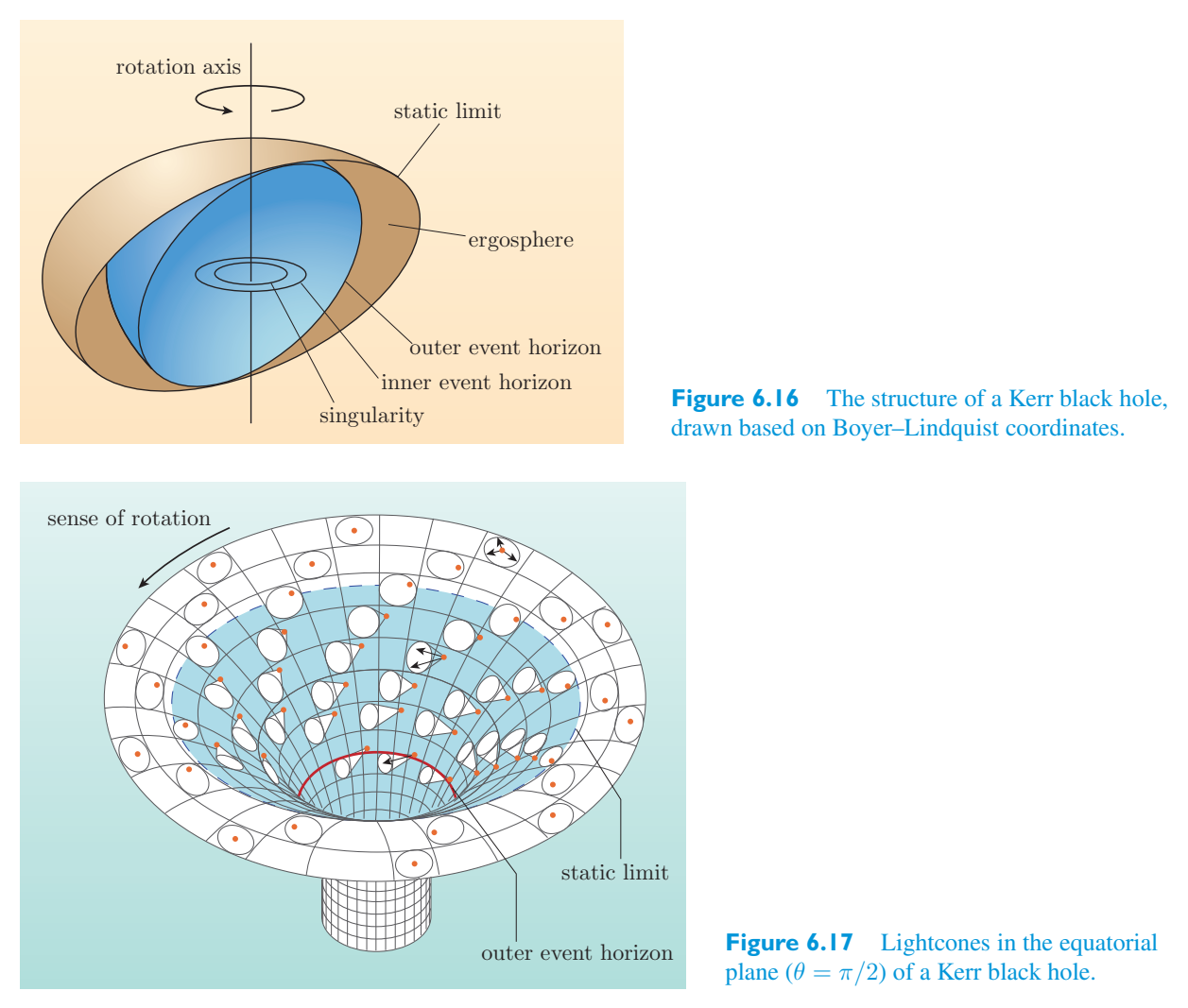
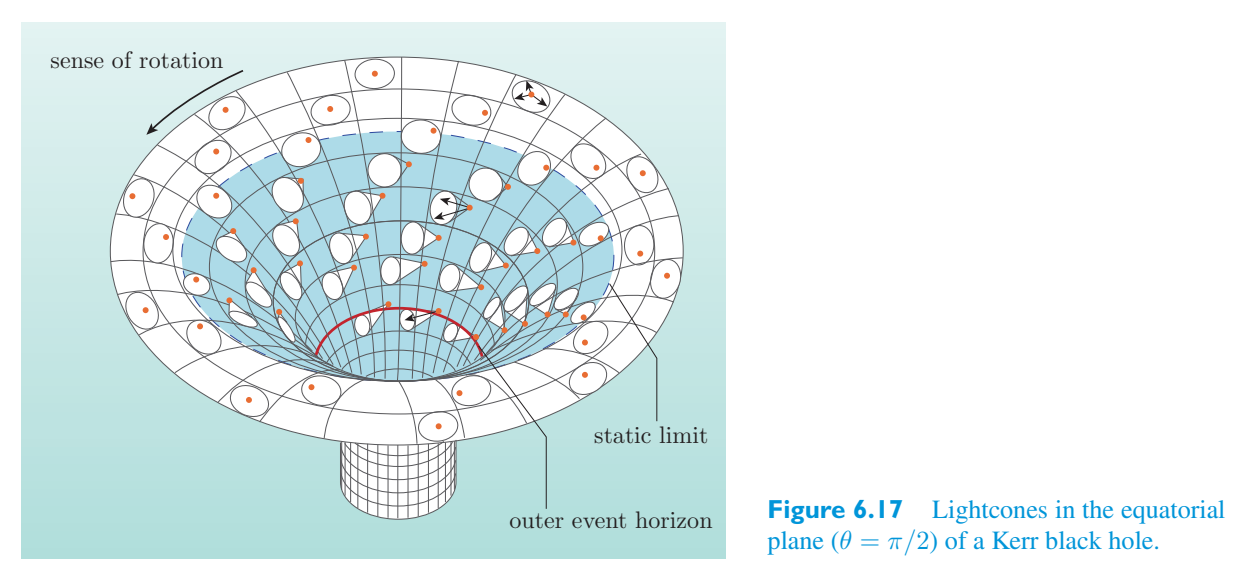
Far from the black hole, light travels with equal ease in all directions. In this asymptotically flat region, lightcones have the usual symmetric form familiar from Minkowski space. Closer to the static limit, the lightcones become increasingly distorted, being tipped towards the origin and tipped in the direction of rotation of the black hole. The static limit marks a particular critical case: imagine a radial line extending from the origin to some point on the static limit and then extending outwards towards the asymptotically flat region. (Any of the radial lines in Figure 6.17 will do.) Now imagine placing a light source on that radial line at the point where it crosses the static limit. As Figure 6.17 indicates, light emitted from that source can travel in directions that take it closer to or further from the origin; it can also travel in directions that take it more-or-less in the direction of rotation of the black hole. What it cannot do is travel in any direction that opposes the direction of rotation of the black hole. At and within the static limit, the skewing of spacetime in the direction of rotation is so strong that motion in the direction of rotation cannot be resisted. Light itself is dragged in that direction, and so, by implication, is anything that travels slower than light. Note that the static limit is not an event horizon; it is quite possible for signals to escape through the static limit, but they must do so by travelling in the direction of rotation. The inability of objects entering the static limit to remain at rest explains why this surface of infinite redshift is called the static limit.远离黑洞,光可以同样轻松地向各个方向传播。在这个渐近平坦的区域中,光锥具有闵可夫斯基空间中常见的对称形式。接近静态极限时,光锥变得越来越扭曲,向原点倾斜并朝黑洞旋转的方向倾斜。静态极限标志着一个特殊的关键情况:想象一条径向线从原点延伸到静态极限上的某个点,然后向外延伸到渐近平坦区域。 (图 6.17 中的任何径向线都可以。)现在想象一下,将光源放置在该径向线上穿过静态限制的点上。如图 6.17 所示,从该光源发出的光可以沿靠近或远离原点的方向传播;它还可以沿着或多或少与黑洞旋转方向相同的方向行进。它不能做的是沿着与黑洞旋转方向相反的任何方向行进。在静态极限内,时空在旋转方向上的倾斜非常强烈,以至于无法抵抗旋转方向上的运动。光本身被拖向那个方向,因此,暗示任何比光传播得慢的东西也是如此。请注意,静态极限不是事件视界;而是事件视界。信号很有可能突破静态限制,但它们必须通过沿旋转方向传播来实现。进入静态极限的物体无法保持静止,这解释了为什么这个无限红移的表面被称为静态极限。
The dragging of inertial frames by a rotating black hole has many consequences. For example, material that starts falling towards the black hole from rest at a great distance will initially move along a radial pathway. However, as it nears the black hole, the effect of frame dragging will increase so, unless it happens to be travelling along the axis of rotation, the in-falling matter will also tend to move in the direction of the black hole’s rotation. Once within the static limit it must move in that direction, irrespective of any action taken to move in the opposite direction.旋转黑洞对惯性系的拖曳会产生许多后果。例如,从远处静止开始落向黑洞的物质最初将沿着径向路径移动。然而,当它接近黑洞时,参考系拖拽的影响会增加,因此,除非它恰好沿着旋转轴行进,否则落入的物质也会倾向于沿着黑洞旋转的方向移动。一旦处于静态限制内,它就必须朝该方向移动,无论采取任何措施朝相反方向移动。
Similarly, photons or other massless particles travelling in the equatorial plane of a rotating black hole will not only be deflected towards the black hole but will also be skewed around the black hole, as indicated in Figure类似地,在旋转黑洞的赤道面中传播的光子或其他无质量粒子不仅会偏向黑洞,而且还会围绕黑洞倾斜,如图所示
6.19.6.19。
Another interesting consequence is the extraction of energy from a rotating black hole through what is known as the Penrose process, originally proposed by Roger Penrose (Figure 6.18) in the 1960s. The process involves some kind of unstable particle that enters the region between the static limit and the outer event horizon, and while there decays to form two other particles. Penrose showed that under appropriate circumstances, including the requirement that one of the particles produced in the decay passes through the outer horizon and enters the black hole, it is possible for the other decay product to pass out through the static limit and carry away more energy from the black hole than the original particle carried in. As a result of the process, the energy and angular momentum of the black hole are reduced, so the process provides a mechanism for extracting rotational energy from the black hole. It is because of this link with energy that the region between the static limit and the outer horizon is called the ergosphere.另一个有趣的结果是通过所谓的彭罗斯过程从旋转黑洞提取能量,该过程最初由 Roger Penrose 在 20 世纪 60 年代提出(图 6.18)。该过程涉及某种不稳定粒子进入静态极限和外部事件视界之间的区域,并在那里衰变形成另外两个粒子。彭罗斯证明,在适当的情况下,包括衰变中产生的一个粒子穿过外视界并进入黑洞的要求,另一种衰变产物有可能穿过静态极限并从黑洞带走比原始粒子携带的更多的能量。由于该过程,黑洞的能量和角动量减少,因此该过程提供了一种从黑洞提取旋转能的机制。正是由于这种与能量的联系,静态极限和外地平线之间的区域被称为能层。
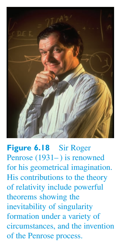
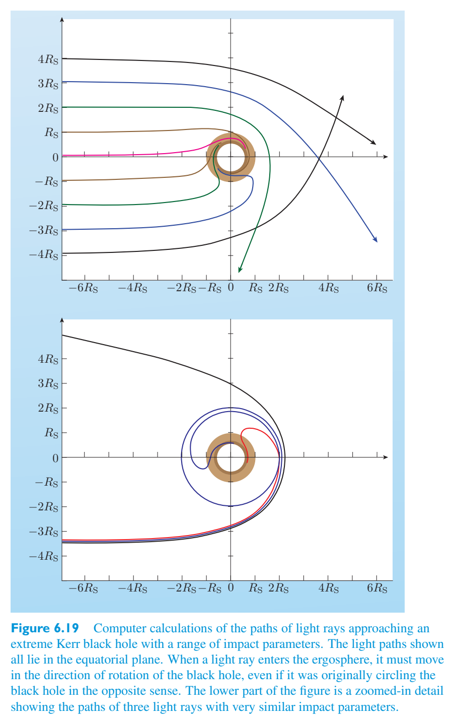
As in the case of the non-rotating black hole, there is much that might be said concerning motion within the outer event horizon. The presence of the inner horizon is a sign of internal complexity, and the introduction of Kruskal-like coordinates leads to a maximal analytic extension that can be interpreted in terms of an infinite sequence of interconnected universes. However, the physical significance of these mathematical features is still unclear so we shall not pursue them here.与非旋转黑洞的情况一样,关于外部事件视界内的运动有很多可说的。内部视界的存在是内部复杂性的标志,类克鲁斯卡尔坐标的引入导致了最大的分析扩展,可以用互连宇宙的无限序列来解释。然而,这些数学特征的物理意义仍然不清楚,所以我们不在这里追究它们。
Exercise 6.8 Consider the representation of a rotating black hole shown in练习 6.8 考虑如图所示的旋转黑洞的表示
Figure 6.20 overleaf. The path of a spacecraft approaching the static limit is shown as a dashed line.图 6.20 背面。航天器接近静态极限的路径显示为虚线。
(a) Explain why this cannot be the path of an observer in free fall.(a) 解释为什么这不可能是观察者自由落体的路径。
(b) Is it possible for the spacecraft to follow the dashed path? Explain.(b) 航天器有可能沿着虚线路径飞行吗?解释。
(c) Is it possible for a spacecraft to follow the dotted path in Figure 6.20? Explain.(c) 航天器是否有可能沿着图 6.20 中的虚线路径飞行?解释。
6.4 Quantum physics and black holes6.4 量子物理和黑洞
Up to this point, all our discussions of black holes have been based on predictions of the general theory of relativity. There is no doubt that black holes exist as solutions to the equations of general relativity, but the existence of ‘real’ black holes is a matter that can be settled only by observation. We shall examine some of the relevant evidence in the next chapter, but even if objects that can be described as black holes do exist, it is possible that parts of physics other than general relativity might significantly influence their properties. In particular, scientists are well aware of the wide importance of quantum phenomena in nature and know of many examples where quantum physics has modified or even completely overthrown the predictions of classical theories such as Newtonian mechanics or Maxwellian electromagnetism. Many physicists look forward to an eventual unification of classical general relativity and quantum physics in a yet to be formulated theory of quantum gravity. Some think that such a unified theory may already be at hand in the form of string theory or the so-called M theory that it has spawned; others strongly disagree. Whatever the fate of M theory, there have already been attempts to use general features of quantum physics that seem likely to survive any future unification to gain insight into the modifications that quantum physics might impose on ‘classical’ black holes. This section is concerned with some of those modifications.到目前为止,我们所有关于黑洞的讨论都是基于广义相对论的预测。毫无疑问,黑洞作为广义相对论方程的解而存在,但“真实”黑洞的存在只能通过观测来解决。我们将在下一章中研究一些相关证据,但即使可以描述为黑洞的物体确实存在,除了广义相对论之外的物理学部分也可能会显着影响它们的性质。特别是,科学家们非常清楚量子现象在自然界中的广泛重要性,并且知道许多量子物理学修改甚至完全推翻牛顿力学或麦克斯韦电磁学等经典理论预测的例子。许多物理学家期待着经典广义相对论和量子物理学最终在尚未制定的量子引力理论中得到统一。一些人认为,这样一个统一的理论可能已经以弦理论或它所衍生的所谓的 M 理论的形式出现了。其他人则强烈反对。无论 M 理论的命运如何,已经有人尝试利用量子物理学的一般特征,这些特征似乎可能在未来的统一中幸存下来,以深入了解量子物理学可能对“经典”黑洞施加的修改。本节涉及其中一些修改。
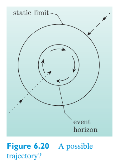
6.4.1 Hawking radiation6.4.1 霍金辐射
In 1975 Stephen Hawking (Figure 6.21) published an influential paper showing that, due to quantum effects, black holes should be sources of radiation. In the paper he demonstrated that a black hole would behave as a body with a finite temperature that was inversely proportional to the mass M of the black hole. The relevant temperature is now called the Hawking temperature, T H, and is given by1975 年,斯蒂芬·霍金(图 6.21)发表了一篇有影响力的论文,表明由于量子效应,黑洞应该是辐射源。在论文中,他证明了黑洞的行为就像一个具有有限温度的物体,该温度与黑洞的质量 M 成反比。相关温度现在称为霍金温度 T H,由下式给出
M中号
where M) = \(2.00\times10^{30}\) kg represents the mass of the Sun, k = \(1.38\times10^{-22}\) \(\mathrm{J\,K^{-1}}\) is the Boltzmann constant, and! = \(1.05\times10^{-34}\) \(\mathrm{J\,s}\) is the Planck constant divided by 2 \(\pi\). The effective temperature of a stellar mass black hole was expected to be very small, but the very idea that a real black hole might act as a thermal source that could radiate away its energy was very striking since it was clearly at odds with the classical concept of a black hole that only ever absorbed radiation. The radiation that would be emitted by a black hole is now known as Hawking radiation.其中 M) = \(2.00\times10^{30}\) kg 表示太阳的质量,k = \(1.38\times10^{-22}\) \(\mathrm{J\,K^{-1}}\) 是玻尔兹曼常数,并且! = \(1.05\times10^{-34}\) \(\mathrm{J\,s}\) 是普朗克常数除以 2 \(\pi\)。恒星质量黑洞的有效温度预计非常小,但真正的黑洞可能充当可以辐射其能量的热源的想法非常引人注目,因为它显然与黑洞仅吸收辐射的经典概念不一致。黑洞发出的辐射现在被称为霍金辐射。
Hawking’s work was originally presented in the highly mathematical context of quantum field theory, but more intuitive interpretations were soon provided. In quantum physics, it was noted, the physical vacuum is subject to quantum fluctuations in which particle–antiparticle pairs can enjoy a short-lived existence before undergoing mutual annihilation. This seething quantum vacuum is not the static, featureless void of classical physics; rather, it is a fluctuating sea of transient particles in which quantum physics allows energy conservation to be violated by an amount \(\Delta E\) for a time interval \(\Delta t\), provided that, roughly, \(\Delta E\) \(\Delta t\) ≤!, as a consequence of Heisenberg’s uncertainty principle.霍金的工作最初是在量子场论的高度数学背景下提出的,但很快就提供了更直观的解释。有人指出,在量子物理学中,物理真空会受到量子涨落的影响,在量子涨落中,粒子-反粒子对可以在相互湮灭之前享受短暂的存在。这种沸腾的量子真空并不是经典物理学中静态的、毫无特征的虚空;它是一种量子真空。相反,它是一个波动的瞬态粒子海洋,其中量子物理学允许在时间间隔 \(\Delta t\) 内违反能量守恒量 \(\Delta E\),前提是,粗略地说,\(\Delta E\) \(\Delta t\) ≤!,这是海森堡测不准原理的结果。
Under normal laboratory circumstances, the effects of the fluctuating quantum vacuum can be measured, but the particles responsible are not directly observed. They are said to be virtual particles since their energy and momentum do not generally satisfy the relation \(E^{2}\) − \(p^{2}\) \(c^2\) = \(m^{2}\) \(c^4\) that applies to real, directly observable particles. It is possible to imagine a virtual particle pair in which one of the pair has positive energy while the other has the corresponding negative energy; such a zero-energy fluctuation might exist according to quantum uncertainty but would be ruled out by the additional requirement that all real particles have positive energy.在正常的实验室环境下,可以测量波动量子真空的影响,但无法直接观察到产生影响的粒子。它们被称为虚粒子,因为它们的能量和动量通常不满足适用于真实的、可直接观察的粒子的关系式 \(E^{2}\) − \(p^{2}\) \(c^2\) = \(m^{2}\) \(c^4\)。可以想象一对虚拟粒子,其中一个具有正能量,另一个具有相应的负能量;根据量子不确定性,这种零能量波动可能存在,但会被所有真实粒子都具有正能量的附加要求所排除。
However, in the extreme conditions close to the event horizon of a black hole, particularly a low-mass black hole where the tidal effect would be very strong and particle–antiparticle pairs might quickly separate, the situation is different. Taking the case of a non-rotating black hole for simplicity, the metric coefficients g = (1 − R/r) and g = (1 − R/r) − 1 change sign at the event horizon, switching the role of space-like and time-like intervals, and allowing particles within the horizon to follow geodesics characterized by negative energy values that would be forbidden outside the horizon. A particle–antiparticle pair, one member of which had a negative energy, might be created just outside the event horizon of a black hole within the limits allowed by quantum uncertainty, and the negative-energy particle might enter the horizon where its negative-energy geodesic is classically allowed. Meanwhile, the positive-energy particle outside the horizon might follow a positive-energy geodesic that would eventually lead to a distant observer. In this way normally short-lived quantum fluctuations might create long-lived observable particles. The positive particle energy measured by a distant observer would be balanced by a negative energy carried into the black hole, so from the point of view of the distant observer there would be no violation of energy conservation. The black hole would emit particles of all kinds and would gradually lose mass as it did so.然而,在接近黑洞事件视界的极端条件下,特别是低质量黑洞,潮汐效应非常强烈,粒子-反粒子对可能会迅速分离,情况就不同了。为了简单起见,以非旋转黑洞为例,度规系数 g = (1 − R/r) 和 g = (1 − R/r) − 1 在事件视界处改变符号,切换类空间和类时间间隔的角色,并允许视界内的粒子遵循以负能量值为特征的测地线,而这在视界外是被禁止的。在量子不确定性允许的范围内,可能会在黑洞的事件视界外产生一对粒子-反粒子对,其中一个成员具有负能量,并且负能量粒子可能会进入其负能量测地线经典允许的视界。与此同时,地平线外的正能量粒子可能会沿着正能量测地线运动,最终到达远处的观察者。通过这种方式,通常短暂的量子涨落可能会产生长寿的可观测粒子。远处观察者测量到的正粒子能量将被带入黑洞的负能量平衡,因此从远处观察者的角度来看,不会违反能量守恒定律。黑洞会发射出各种粒子,并在此过程中逐渐失去质量。
Of course, this intuitive argument does not account for details such as the Hawking temperature or the thermal spectrum of Hawking radiation, but it can be extended to make such outcomes plausible. What it does do is indicate the potential interplay of quantum physics and classical general relativity.当然,这种直观的论证并没有考虑霍金温度或霍金辐射的热谱等细节,但它可以扩展以使这样的结果变得合理。它的作用是表明量子物理学和经典广义相对论之间潜在的相互作用。
In classical physics an ideal thermal source of electromagnetic radiation (a black body) of surface area A and temperature T emits energy at a rate proportional to AT 4. For a Schwarzschild black hole, A ∝ \(R^2\) ∝ M 2 and T = T ∝ 1/M, so the rate of energy emission by Hawking radiation is在经典物理学中,表面积为 A、温度为 T 的理想电磁辐射热源(黑体)以与 AT 4 成比例的速率发射能量。对于史瓦西黑洞,A ∝ \(R^2\) ∝ M 2 且 T = T ∝ 1/M,因此霍金辐射的能量发射速率为
So, as the mass of the black hole decreases, its rate of energy emission will accelerate, causing a low-mass black hole (if such an object exists) to end its life with an escalating burst of energy emission that would be seen as an explosion! Such explosions are improbable because most black holes are likely to increase their mass by accreting matter from their environment. Nonetheless it is interesting to determine the expected life of an isolated black hole.因此,随着黑洞质量的减小,其能量发射的速度将会加快,导致低质量黑洞(如果存在这样的物体)以不断升级的能量发射爆发结束其生命,这将被视为爆炸!这种爆炸是不可能的,因为大多数黑洞很可能通过吸积环境中的物质来增加其质量。尽管如此,确定孤立黑洞的预期寿命还是很有趣的。
To a distant observer, the emission of energy \(\Delta E\) is compensated by a decrease of − \(\Delta M =\)\(\Delta E\)/\(c^2\) in the mass of the black hole. Thus对于远处的观察者来说,能量的发射 \(\Delta E\) 通过黑洞质量的减少 - \(\Delta M =\)\(\Delta E\)/\(c^2\) 来补偿。因此
The solution of the corresponding differential equation implies that a black hole of current mass M has a remaining lifetime proportional to M 3. In fact, the approximate total lifetime of an isolated black hole is estimated to be相应微分方程的解意味着当前质量为 M 的黑洞的剩余寿命与 M 3 成正比。事实上,孤立黑洞的总寿命大约为
The above takes account of the emission of photons; the production of other particles does not affect the dependence on mass, only the constant of M < \(10^{22}\) kg that loses proportionality. The lifetime \(\tau\) of a black hole of mass mass by radiating only photons and neutrinos is given by上述考虑了光子的发射;其他粒子的产生不会影响对质量的依赖性,只有 M < \(10^{22}\) kg 的常数会失去比例性。仅辐射光子和中微子的质量质量黑洞的寿命 \(\tau\) 由下式给出
Hence an isolated mini black hole of mass \(2\times10^{11}\) kg, formed during the Big Bang say, might now be in its death throes.因此,在大爆炸期间形成的质量为 \(2\times10^{11}\) kg 的孤立迷你黑洞现在可能正处于垂死挣扎。
Exercise 6.9 Why would the discovery of a mini black练习 6.9 为什么迷你黑的发现会
hole be important for physics?空穴对物理学很重要吗?
6.4.2 Singularities and quantum physics6.4.2 奇点和量子物理
In 1965 Roger Penrose showed that all massive bodies surrounded by an event horizon must contain a gravitational singularity that cannot be eliminated by a clever choice of coordinates. Although the singularity is hidden from outside observers by the event horizon, one identifying feature is that the curvature tensor generates an invariant scalar quantity that diverges and approaches infinity at the singularity. Once anything penetrates the event horizon, its world-line ends up at the singularity with no overshoot. Geodesics come to an end at finite values of their affine parameters in a region of finite mass but zero volume.1965 年,罗杰·彭罗斯 (Roger Penrose) 证明,所有被事件视界包围的大质量物体都必须包含一个引力奇点,而这个引力奇点无法通过巧妙选择坐标来消除。尽管事件视界对外部观察者隐藏了奇点,但一个识别特征是曲率张量生成一个不变标量,该标量在奇点处发散并接近无穷大。一旦任何物体穿透事件视界,它的世界线就会在奇点处结束,而不会出现超调。测地线在质量有限但体积为零的区域中以仿射参数的有限值结束。
Although general relativity implies infinite density, many physicists suspect that quantum physics might somehow prevent such singularities from forming. A number of specific mechanisms have been advanced but there is no general agreement about this at the present time. On very general grounds it is expected that quantum effects and gravitational effects will become comparable at the Planck scale, which is characterized by尽管广义相对论意味着无限密度,但许多物理学家怀疑量子物理学可能会以某种方式阻止这种奇点的形成。已经提出了一些具体机制,但目前对此尚未达成普遍共识。从非常普遍的角度来看,预计量子效应和引力效应将在普朗克尺度上变得具有可比性,其特点是
- • Planck energy E = (! c 5/G) 1/2 = \(1.22\times10^{19}\) GeV• 普朗克能量 E = (!c 5/G) 1/2 = \(1.22\times10^{19}\) GeV
- • Planck length l = (! G/\(c^3\)) 1/2 = \(1.62\times10^{-36}\) m• 普朗克长度 l = (!G/\(c^3\)) 1/2 = \(1.62\times10^{-36}\) m
- • Planck time t = (! G/c 5) 1/2 = \(5.39\times10^{-44}\) s.• 普朗克时间t = (!G/c 5) 1/2 = \(5.39\times10^{-44}\) 秒。
The Planck units are usually taken to represent the natural domain of quantum gravity, but they are currently far beyond our capacity for direct experimental investigation. If it is only at these extreme scales that the classical view of singularity becomes untenable, then the non-existence of ideal classical singularities might be of little astronomical significance. Supermassive black holes accreting a few solar masses of matter per year could still account for the energy emission from quasars, and lesser amounts of matter being heated to million degree temperatures in a swirling disc around a stellar mass black hole would still account for the intense X-ray sources not explained by neutron stars. Nonetheless an understanding of quantum gravity that included a quantum theory of spacetime singularities could hold many surprises and so it remains one of the main aims of gravitational research.普朗克单位通常被用来代表量子引力的自然领域,但它们目前远远超出了我们直接实验研究的能力。如果只有在这些极端尺度上,奇点的经典观点才变得站不住脚,那么理想的经典奇点的不存在可能没有什么天文学意义。超大质量黑洞每年吸积几个太阳质量的物质仍然可以解释类星体的能量发射,而在恒星质量黑洞周围的旋转盘中被加热到百万度温度的少量物质仍然可以解释中子星无法解释的强X射线源。尽管如此,对包括时空奇点量子理论在内的量子引力的理解可能会带来许多惊喜,因此它仍然是引力研究的主要目标之一。
Summary of Chapter 6第 6 章总结
1. According to classical general relativity, a black hole is a region of1. 根据经典广义相对论,黑洞是一个区域
spacetime that matter and radiation may enter but from which they may not escape. The region is bounded by an event horizon that separates events that can be seen by an external observer from those that cannot be seen. At the heart of a black hole is a gravitational singularity at which invariant quantities related to the curvature of spacetime diverge.物质和辐射可以进入但无法逃脱的时空。该区域以事件视界为界,将外部观察者可以看到的事件与无法看到的事件分开。黑洞的中心是一个引力奇点,与时空曲率相关的不变量在此处发散。
2. Singularities may arise from the complete gravitational collapse of massive2. 奇点可能是由于大质量物体的完全引力塌缩而产生的
bodies such as degenerate stars (white dwarfs and neutron stars) that have exceeded their limiting mass, or even, much more speculatively, from smaller bodies compressed by cosmological processes in the early Universe.诸如简并星(白矮星和中子星)等超过其极限质量的天体,或者甚至更推测,来自早期宇宙中被宇宙学过程压缩的较小天体。
3. Black holes are commonly classified according to their mass or according to3. 黑洞通常根据其质量或根据
the solution of the vacuum field equations that describes them. The only independent externally measurable properties of a black hole are its mass, charge and angular momentum.描述它们的真空场方程的解。黑洞唯一可独立外部测量的属性是其质量、电荷和角动量。
4. Supermassive black holes might account for the energy emitted by quasars4. 超大质量黑洞可能是类星体释放能量的原因
and other forms of active galaxy. Stellar mass black holes might account for some stellar sources of X-rays, though others can be accounted for by the action of neutron stars.以及其他形式的活跃星系。恒星质量黑洞可能可以解释一些X射线的恒星源,尽管其他的可以通过中子星的作用来解释。
5. A non-rotating black hole is described by the stationary, spherically5. 非旋转黑洞被描述为静止的、球形的
symmetric, Schwarzschild solution of the Einstein vacuum field equations. In Schwarzschild coordinates the solution has a gravitational singularity at r = 0 and a coordinate singularity at r = R = 2 GM/\(c^2\), the Schwarzschild radius, which is also the location of the event horizon.爱因斯坦真空场方程的对称史瓦西解。在史瓦西坐标中,解在 r = 0 处有一个引力奇点,在 r = R = 2 GM/\(c^2\) 处有一个坐标奇点,史瓦西半径,也是事件视界的位置。
6. A body released from rest at a large distance from a non-rotating black hole6. 距离非旋转黑洞很远的地方从静止状态释放出来的物体
only requires a finite proper time to fall freely to the central singularity. Nothing unusual happens to the body as it passes through the event horizon, though this marks a point of no return on the inward motion of the body. Once within the horizon the body will inevitably reach the central singularity.只需要有限的本征时间就可以自由落体到中心奇点。当物体穿过事件视界时,没有发生任何异常情况,尽管这标志着物体向内运动的一个不归路。一旦进入视界,物体将不可避免地到达中心奇点。
7. As seen by a distant stationary observer, a body falling into a black hole7. 正如一个遥远的静止观察者所看到的,一个物体落入黑洞
takes an infinite amount of coordinate time to reach the event horizon. Light signals emitted from the object also take an increasing amount of需要无限量的坐标时间才能到达事件视界。从物体发出的光信号也需要越来越多的光信号
(coordinate) time to reach a distant observer. These effects reduce the rate at which photons from the falling body reach the distant observer (for whom coordinate time and proper time agree) and contribute to an observed dimming of the body.(坐标)到达远处观察者的时间。这些效应降低了下落物体的光子到达远处观察者(坐标时间和本征时间一致)的速率,并导致观察到的物体变暗。
8. Signals from the falling body are redshifted according8. 下落物体发出的信号根据以下公式发生红移
to the distant observer, with the horizon representing a surface of infinite redshift. This reduces the energy per photon received by the distant observer and further contributes to the observed dimming.对于远处的观察者来说,地平线代表无限红移的表面。这减少了远处观察者接收到的每个光子的能量,并进一步导致观察到的变暗。
9. Bodies in the neighbourhood of a black hole are subject9. 黑洞附近的物体受到影响
to tidal effects that arise from the presence of spacetime curvature and are described by the equation of geodesic deviation. These effects can be lethal outside the event horizon of a stellar mass black hole but would be mild at the event horizon of a supermassive black hole.由于时空曲率的存在而产生的潮汐效应,并由测地偏差方程描述。这些影响在恒星质量黑洞的事件视界之外可能是致命的,但在超大质量黑洞的事件视界内却是温和的。
10. There would be a strong gravitational deflection of10. 将会产生强烈的引力偏转
light close to a black hole with photons having the possibility of entering an (unstable) circular orbit at the radius of the photon sphere, 1.5 \(R_S\).靠近黑洞的光,其光子有可能进入光子球半径 1.5 \(R_S\) 的(不稳定)圆形轨道。
11. Lightcones and spacetime diagrams provide valuable11. 光锥和时空图提供了有价值的信息
tools for investigating local spacetime structure in general relativity, but the behaviour of lightcones will depend on the particular coordinates being used. In Schwarzschild coordinates lightcones show abrupt changes at the Schwarzschild radius, which marks a coordinate singularity. Advanced Eddington–Finkelstein coordinates remove the coordinate singularity and produce lightcones that change in a regular way, tipping and narrowing as they approach the Schwarzschild radius. The behaviour of the lightcones at and within the Schwarzschild radius indicates the inevitability of encountering the central singularity, though more powerful methods must be used to prove that inevitability.用于研究广义相对论中局部时空结构的工具,但光锥的行为将取决于所使用的特定坐标。在史瓦西坐标中,光锥显示史瓦西半径处的突变,这标志着坐标奇点。高级爱丁顿-芬克尔斯坦坐标消除了坐标奇点并产生以规则方式变化的光锥,当它们接近史瓦西半径时倾斜和变窄。史瓦西半径处和之内的光锥的行为表明遇到中心奇点的必然性,尽管必须使用更强大的方法来证明这种必然性。
12. A rotating black hole is characterized by a mass M12. 旋转黑洞的特征是质量 M
and an angular momentum magnitude J = M ac, and is described by the stationary, axi-symmetric Kerr solution of the Einstein vacuum field equations. In Boyer–Lindquist coordinates the solution has a central ring-shaped gravitational singularity of radius a, and coordinate singularities at the ellipsoidal surfaces角动量大小 J = M ac,由爱因斯坦真空场方程的平稳轴对称克尔解描述。在 Boyer-Lindquist 坐标中,解具有半径为 a 的中心环形引力奇点,并且坐标奇点位于椭球面
which behave as outer and inner event horizons.它们表现为外部和内部事件视界。
13. The ellipsoidal surface13. 椭球面
is a surface of infinite redshift that encloses the outer event horizon, meeting it only at the poles (except in the case of an extreme Kerr black hole, when both surfaces are coincident spheres).是一个无限红移的表面,包围着外部事件视界,仅在两极相交(极端克尔黑洞的情况除外,此时两个表面都是重合的球体)。
14. The surface s + also marks the static limit, within which all particles must14. 表面 s+ 也标志着静态极限,在该极限内所有颗粒必须
move in the direction of rotation of the black hole.沿着黑洞的旋转方向移动。
15. The motion of massive bodies and light rays in the neighbourhood of a15. 物体附近的大质量物体和光线的运动
rotating black hole is skewed in the direction of rotation of the black hole as a consequence of the dragging of inertial frames by the black hole.由于黑洞拖动惯性系,旋转黑洞在黑洞旋转方向上发生倾斜。
16. Quantum physics may cause the properties of real black holes to differ16. 量子物理学可能会导致真实黑洞的属性有所不同
significantly from those of black holes in classical general relativity. In particular, Hawking radiation may allow black holes to act as thermal sources of radiation with a Hawking temperature that is inversely proportional to the mass of the black hole. If so, the explosion of isolated (mini) black holes is possible, though unlikely due to the greater probability of the accretion of mass from the surrounding environment. Quantum physics might also prevent the formation of ideal classical singularities, though this will not necessarily affect the ability of black holes to account for the energetic emissions from various galactic and stellar sources.与经典广义相对论中的黑洞有很大不同。特别地,霍金辐射可以允许黑洞充当辐射热源,其霍金温度与黑洞的质量成反比。如果是这样,孤立(微型)黑洞的爆炸是可能的,尽管由于周围环境质量吸积的可能性较大,这种可能性不大。量子物理学也可能阻止理想经典奇点的形成,尽管这不一定会影响黑洞解释各种星系和恒星源的能量发射的能力。
Chapter 7 Testing general relativity第7章检验广义相对论
Introduction介绍
Up to this point, our discussion of general relativity has been mainly theoretical. This chapter concerns the experimental and observational evidence regarding general relativity. We start with the so-called ‘classic tests’, interpreting that term in its most liberal sense to include some experiments that were not performed until the early 1960s. We draw the dividing line at that point to separate those early tests from a number of more recent satellite-based tests, and astronomical observations of presumed black holes and gravitational lenses. We end with a section on gravitational waves. This last topic might well have been a chapter in its own right, but the theory of gravitational waves is too sophisticated to be treated fully in this book, while the observational aspects are too important to overlook. For that reason the topic is mainly treated as an observational one but is given an unusually detailed theoretical introduction.到目前为止,我们对广义相对论的讨论主要是理论上的。本章涉及广义相对论的实验和观测证据。我们从所谓的“经典测试”开始,从最自由的意义上解释该术语,包括一些直到 20 世纪 60 年代初才进行的实验。我们在这一点上划出了分界线,将这些早期测试与一些最近的基于卫星的测试以及假定的黑洞和引力透镜的天文观测分开。我们以引力波部分结束。最后一个主题很可能本身就是一章,但引力波理论太复杂,无法在本书中充分讨论,而观测方面又太重要,不容忽视。因此,该主题主要被视为观察性主题,但给出了异常详细的理论介绍。
There have been many references to tests and observations in earlier chapters. Where appropriate this chapter refers back to the material that inspired them and where necessary builds on it.前面的章节中多次提到了测试和观察。本章在适当的情况下回顾了激发他们灵感的材料,并在必要时建立在这些材料的基础上。
7.1 The classic tests of general relativity7.1 广义相对论的经典检验
7.1.1 Precession of the perihelion of Mercury7.1.1 水星近日点的进动
A famous prediction of Newtonian mechanics is that the path of an isolated planet moving around the Sun is an ellipse, with the Sun at one focus of the ellipse, as illustrated in Figure 7.1. As well as having a specific size (described by its semi-major axis, a) and a specific shape (described by its eccentricity, e), an elliptical orbit also has a specific orientation in the orbital plane. This orientation can be specified by the direction of the line joining the Sun to the point of closest approach of the planet; this point is called the perihelion. According to Newtonian mechanics, for a spherically symmetric Sun and an isolated planet, this direction should not change — the planet’s perihelion should occur at the same point in space, orbit after orbit.牛顿力学的一个著名预测是,一颗孤立的行星绕太阳运行的路径是一个椭圆,太阳位于椭圆的一个焦点上,如图7.1所示。除了具有特定的尺寸(由其半长轴 a 描述)和特定的形状(由其偏心率 e 描述)之外,椭圆轨道还在轨道平面中具有特定的方向。这个方向可以通过联络太阳到最接近行星的点的线的方向来指定;该点称为近日点。根据牛顿力学,对于球对称的太阳和孤立的行星,这个方向不应该改变——行星的近日点应该出现在太空中的同一点,一个又一个轨道。
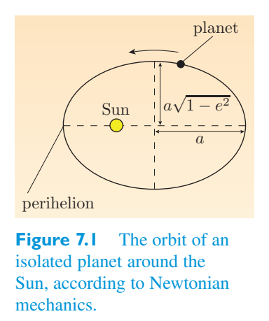
By 1845 it was known that the orbit of the planet Mercury did not behave in this way. With each successive orbit, the orbital orientation changed slightly, as shown in exaggerated form in Figure 7.2. This movement is called perihelion precession; a large part of it can be accounted for by using Newtonian mechanics to calculate the gravitational effect on Mercury of the other planets. However, by 1859 the work of Urbain Le Verrier (1811–1877) had shown that there was a small but significant residual movement, amounting to 43 seconds of arc per century, that could not be accounted for by any known Newtonian force. In spite of much effort over many years (including some fairly wild conjectures), no satisfactory reason for the residual precession could be found. Then in 1915, Einstein, using what would later be seen as an approximate form of the Schwarzschild metric, showed that general relativity predicts a perihelion advance of just the right amount. This was an important early triumph for the theory that did much to convince Einstein that he was on the right track.到 1845 年,人们知道水星的轨道并非如此。对于每个连续的轨道,轨道方向都会略有变化,如图 7.2 中放大的形式所示。这种运动称为近日点进动;其中很大一部分可以通过使用牛顿力学计算其他行星对水星的引力效应来解释。然而,到 1859 年,乌尔班·勒维耶 (Urbain Le Verrier,1811-1877) 的工作表明,存在着微小但显着的残余运动,相当于每世纪 43 弧秒,任何已知的牛顿力都无法解释这一现象。尽管多年来付出了很多努力(包括一些相当疯狂的猜想),但仍无法找到剩余进动的令人满意的原因。然后在 1915 年,爱因斯坦使用后来被视为史瓦西度规的近似形式,表明广义相对论预测近日点的前进量恰到好处。这是该理论的一个重要的早期胜利,它极大地说服了爱因斯坦,他走在正确的道路上。
The changing orientation of orbits in general relativity was mentioned at the end of Chapter 5, in the context of the Schwarzschild solution, where it was associated with an additional non-Newtonian term in the orbital shape equation. It can be shown that for each orbit, the perihelion advances by an angle Δ \(\phi\) given by广义相对论中轨道方向的变化在第 5 章末尾在史瓦西解的背景下提到,其中它与轨道形状方程中的附加非牛顿项相关。可以证明,对于每个轨道,近日点前进的角度为 Δ \(\phi\),由下式给出
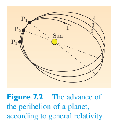
where M is the total mass of the system (in this case dominated by that of the Sun), a is the semi-major axis, and e is the eccentricity. (A circular orbit has e = 0.) Clearly, Δ \(\phi\) becomes larger as a becomes smaller and as e approaches 1. Mercury has an orbit with high eccentricity and a small semi-major axis so it is a good candidate for measuring the advance of the perihelion. The original observations were carried out by means of optical telescopes but now radar ranging is used for greater precision. This enables the effect of general relativity on the precession of the perihelion of other planets (including the minor body Icarus) to be tested, as shown in Table 7.1.其中 M 是系统的总质量(在本例中主要是太阳的质量),a 是半长轴,e 是偏心率。 (圆形轨道的 e = 0。)显然,随着 a 变小以及 e 接近 1,Δ \(\phi\) 会变大。水星的轨道偏心率高,半长轴小,因此它是测量近日点前进的良好候选者。最初的观测是通过光学望远镜进行的,但现在使用雷达测距来提高精度。这样就可以测试广义相对论对其他行星(包括小天体伊卡洛斯)近日点进动的影响,如表7.1所示。
Exercise 7.1 Mercury has a period of 87.969 days, semi-major axis练习 7.1 水星的周期为 87.969 天,半长轴
a = \(5.791\times10^{10}\) m and eccentricity e = 0.2067, and the mass of the Sun is M) = \(1.989\times10^{30}\) kg. Calculate the general relativistic contribution to the rate of perihelion precession. Express your answer in seconds of arc per century.a = \(5.791\times10^{10}\) m,偏心率 e = 0.2067,太阳质量为 M) = \(1.989\times10^{30}\) kg。计算广义相对论对近日点进动速率的贡献。以每世纪弧秒表示你的答案。
Table 7.1 Predicted and observed rates of residual perihelion advance in seconds of arc per century for various planets and for the minor body Icarus.表 7.1 各个行星和小天体伊卡洛斯的预测和观测的残余近日点前进率(以弧秒为单位)。
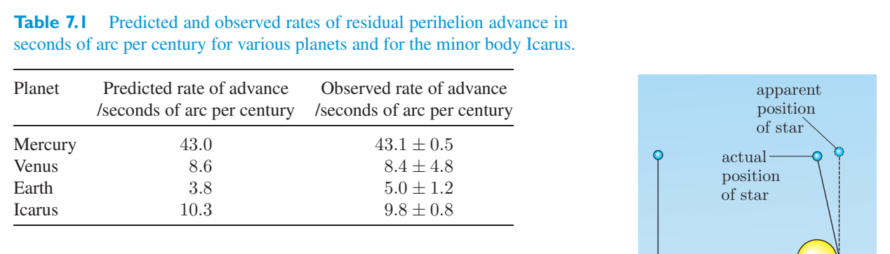
7.1.2 Deflection of light by the Sun7.1.2 太阳对光的偏转
The second testable prediction of general relativity concerns the deflection of light by a massive body. This was noted by Einstein as a general consequence of the principle of equivalence, and we saw in the previous chapter the extreme case of deflected light paths in the neighbourhood of rotating and non-rotating black holes. In the case of light rays passing close to the limb (i.e. the edge) of the Sun, the effect is small but large enough to be detectable. The effect is illustrated schematically in Figure 7.3.广义相对论的第二个可检验的预测涉及大质量物体对光的偏转。爱因斯坦指出这是等效原理的一般结果,我们在前一章中看到了旋转和非旋转黑洞附近光路偏转的极端情况。在光线靠近肢体的情况下(即,太阳的边缘),影响很小,但大到足以被检测到。其效果如图 7.3 所示。
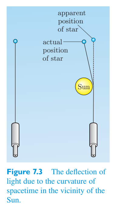
Using the null geodesics of the Schwarzschild metric to represent the world-lines of light rays that pass close to a spherically symmetric body of mass, general relativity predicts that the angle of deflection Δ \(\theta\) is given (in radians) by使用史瓦西度规的零测地线来表示穿过球对称质量体的光线的世界线,广义相对论预测偏转角 Δ \(\theta\) 由下式给出(以弧度为单位):
where b is the impact parameter (i.e. the perpendicular distance from the initial path of the light ray to the deflecting body). We can see that this effect is largest when b is as small as possible, which occurs for rays just grazing the massive body.其中b是影响参数(即从光线初始路径到偏转体的垂直距离)。我们可以看到,当 b 尽可能小时,这种效应最大,这种情况发生在光线刚刚掠过大质量物体的情况下。
Exercise 7.2 Use Equation 7.2 to calculate the deflection练习 7.2 使用公式 7.2 计算挠度
(in seconds of arc) for rays just grazing the limb of the Sun.(以弧秒为单位)用于刚刚掠过太阳边缘的光线。
The first problem in trying to verify this prediction is that it’s not easy to see any stars at all when the Sun is above the horizon, and it is particularly difficult to see stars that appear just beyond the edge of the Sun’s disc. Observing such stars during a total eclipse of the Sun, when the Moon is directly between the Earth and the Sun, eliminates most of the unwanted sunlight. However, a considerable number of experimental difficulties remain, not the least of which is poor weather conditions on the Earth during the 7 1 minutes maximum total eclipse time. Table 7.2 lists some attempts at this measurement. In spite of the experimental difficulties, it was the expeditions planned by Sir Arthur Eddington (the first two entries in this table) that gave general relativity its most publicized initial triumph and made Einstein a world-famous figure.试图验证这一预测的第一个问题是,当太阳位于地平线以上时,根本不容易看到任何恒星,尤其是看到出现在太阳圆盘边缘之外的恒星尤其困难。当月球直接位于地球和太阳之间时,在日全食期间观察这些恒星可以消除大部分不需要的阳光。然而,仍然存在相当多的实验困难,其中最重要的是在 7 分 1 分钟的最大日全食时间期间地球的恶劣天气条件。表 7.2 列出了此测量的一些尝试。尽管存在实验困难,但阿瑟·爱丁顿爵士计划的探险活动(本表中的前两项)使广义相对论获得了最广为人知的初步胜利,并使爱因斯坦成为世界著名人物。
There seems to be little scope for improving these measurements; for example, a这些测量结果似乎没有什么改进的余地;例如,一个
0.11 times the prediction预测值的0.11倍
measurement in 1975 gave a deflection that was 0.95 ± of general relativity, which is consistent, but hardly a precision confirmation. Such optical measurements have been superseded by radio interferometry. The idea is that by using two radio telescopes, one can measure the very small differences between the times that particular wave crests arrive at the two observatories. The resolution is proportional to the distance between the radio telescopes and this has led to the development of very long baseline interferometry (VLBI), involving two or more observatories, often separated by thousands of kilometres, emulating one giant telescope. Using radio transmission from certain quasars (which are so distant as to be almost point sources of radio waves) and measuring the deflection as the source is eclipsed by the Sun, the predicted gravitational deflection has been verified to better than 0.04%.1975 年的测量给出了广义相对论的 0.95 ± 偏转,这是一致的,但很难得到精确的确认。这种光学测量已被无线电干涉测量法所取代。这个想法是,通过使用两台射电望远镜,人们可以测量特定波峰到达两个天文台的时间之间非常小的差异。分辨率与射电望远镜之间的距离成正比,这导致了超长基线干涉测量(VLBI)的发展,涉及两个或多个天文台,通常相距数千公里,模拟一台巨型望远镜。利用某些类星体(距离很远,几乎是无线电波的点源)的无线电传输并测量源被太阳遮蔽时的偏转,预测的引力偏转已被验证优于 0.04%。
7.1.3 Gravitational redshift and gravitational7.1.3 引力红移和引力
time dilation时间膨胀
The third testable prediction of general relativity concerns gravitational time dilation and the related gravitational redshift. This effect was also predicted at an early stage in the development of general relativity, based on the principle of equivalence. A detailed quantitative prediction for a stationary emitter and a stationary observer was given in Chapter 5 using the Schwarzschild metric. The general relationship obtained there was广义相对论的第三个可检验的预测涉及引力时间膨胀和相关的引力红移。在广义相对论发展的早期阶段,基于等效原理也预测了这种效应。第 5 章使用史瓦西度规对静止发射器和静止观测器进行了详细的定量预测。那里得到的一般关系是
where \(dt_{\rm em}\) represents the coordinate time separating two events at the location of the stationary emitter, and \(d\tau_{\rm ob}\) is the proper time separating sightings of those two events by a stationary observer at radial coordinate position \(r_{\rm ob}\). When the observer is far away, so that \(r_{\rm ob}\) → ∞, we can represent其中 \(dt_{\rm em}\) 表示在静止发射器位置处分隔两个事件的坐标时间,\(d\tau_{\rm ob}\) 是在径向坐标位置 \(r_{\rm ob}\) 处的静止观察者观测到这两个事件的固有时间。当观察者距离较远时,使得\(r_{\rm ob}\)→∞,我们可以表示
Table 7.2 History of observations of light bending, 1919-52. (Source: Sciama, D.W. (1972) The Physical Foundation of General Relativity, Heinemann Educational Books.)表 7.2 光弯曲观测历史,1919-52。 (来源:Sciama, D.W. (1972) 广义相对论的物理基础,Heinemann 教育书籍。)
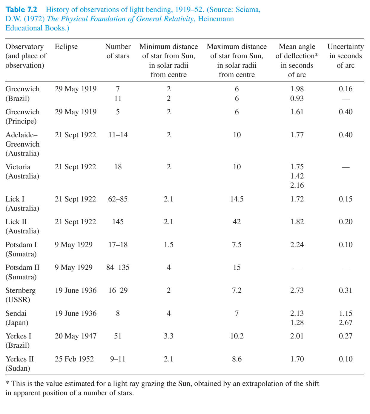
At the location of the emitter, where r = \(r_{\rm em}\),在发射器的位置,其中 r = \(r_{\rm em}\),
so we get the following relation between the proper time separating events at the receiver and the proper time separating their sighting by the distant observer:因此,我们得到接收器处的事件间隔的本征时间与远处观察者的观测间隔的本征时间之间的关系:
Since frequency is inversely proportional to period, we arrive at the following prediction concerning the gravitational redshift in the radiation from a stationary emitter:由于频率与周期成反比,因此我们得出以下关于静止发射器辐射中的引力红移的预测:
It was hoped that this effect would be seen in the spectra of stars, as a reduction in the observed frequency of spectral lines. In fact, in the 1916 paper that contained the first complete formulation of general relativity, Einstein referred to the astronomer Erwin Freundlich, saying:人们希望这种效应能够在恒星的光谱中看到,即观测到的谱线频率的减少。事实上,在 1916 年包含第一个完整的广义相对论公式的论文中,爱因斯坦提到了天文学家欧文·弗罗因德利希 (Erwin Freundlich),他说:
According to E Freundlich, spectroscopical observations on fixed stars of certain types indicate the existence of an effect of this kind, but a crucial test of this consequence has not yet been made.根据弗罗因德利希的说法,对某些类型恒星的光谱观测表明存在这种效应,但尚未对这种结果进行关键测试。
Unfortunately, such a test was very difficult to perform. Early attempts based on normal stars were inconclusive. The spectra were easy to observe, but the anticipated gravitational redshift turned out to be small compared with other effects, such as Doppler shifts due to turbulence in the star’s atmosphere. Observing the spectra of dense stars (where M is relatively large and \(r_{\rm em}\) is relatively small) provided better prospects of success. The first white dwarf was discovered in 1910 — attention was drawn to it in 1914 — and a second white dwarf, the companion to Sirius, was found by the American astronomer Walter Adams in 1915. Eddington emphasized the exceptional density of these stars in the 1920s and pointed out the large gravitational redshift that they should exhibit. In 1925, careful measurements by Adams confirmed these expectations but the ‘test’ was not very precise. More precise astronomical measurements were eventually performed but only after gravitational redshift had been used in the first precise laboratory-based test of general relativity.不幸的是,这样的测试很难进行。基于普通恒星的早期尝试没有结果。光谱很容易观察到,但与其他效应(例如恒星大气湍流引起的多普勒频移)相比,预期的引力红移很小。观测致密恒星的光谱(其中 M 相对较大,rem 相对较小)提供了更好的成功前景。第一颗白矮星于 1910 年被发现,并于 1914 年引起人们的注意。美国天文学家沃尔特·亚当斯于 1915 年发现了第二颗白矮星,即天狼星的伴星。爱丁顿在 1920 年代强调了这些恒星的异常密度,并指出它们应该表现出巨大的引力红移。 1925 年,亚当斯的仔细测量证实了这些预期,但“测试”并不十分精确。最终进行了更精确的天文测量,但只有在引力红移被用于第一个基于实验室的精确广义相对论测试之后。
The Pound–Rebka experiment庞德-雷布卡实验
In 1960, Robert Pound (1919–) and Glen Rebka (1931–) published the results of a terrestrial measurement of gravitational redshift. Before describing the experiment itself, let’s examine the theoretical basis of the test. If we use m to represent the mass of the Earth and f r to represent the proper frequency of an emitter located at coordinate radius r (measured from the centre of the Earth), the gravitational redshift relationship of Equation 5.17 tells us that1960 年,罗伯特·庞德 (Robert Pound,1919–) 和格伦·雷布卡 (Glen Rebka,1931–) 发表了地面引力红移测量结果。在描述实验本身之前,我们先来看看该测试的理论基础。如果我们用 m 代表地球的质量,用 fr 代表位于坐标半径 r(从地球中心测量)的发射器的固有频率,则方程 5.17 的引力红移关系告诉我们:
and for the values of interest this is well approximated by the relation对于感兴趣的值,这可以很好地近似为以下关系
We now want to relate the frequency of light emitted from the original point at coordinate radius r to the frequency of light received at some different point with radial coordinate r + h. The best way to think of this is to imagine a train of waves with period \(\Delta \tau\) r at radius r and period \(\Delta t\) at a point at infinity, i.e. \(\Delta t\) is the coordinate time interval corresponding to \(\Delta \tau\) r. At whatever radius the radiation is received, the coordinate time interval (and its reciprocal f ∞) will be the same, so f r + h, the measured frequency at radius r + h, must be现在我们想要将从坐标半径为 r 的原始点发出的光的频率与在半径坐标为 r + h 的某个不同点接收到的光的频率相关联。考虑这一点的最佳方法是想象一列波,其半径为 r 的周期为 \(\Delta \tau\) r,无穷远点的周期为 \(\Delta t\),即 \(\Delta t\) 是对应于 \(\Delta \tau\) r 的坐标时间间隔。无论接收到的辐射半径如何,坐标时间间隔(及其倒数 f ∞)都将相同,因此 f r + h(半径 r + h 处的测量频率)必须为
If h is small, then a first-order Taylor expansion shows that the frequency measured at r + h differs from f r by如果 h 很小,则一阶泰勒展开表明,在 r + h 处测量的频率与 f r 的差异为
Using Equation 7.4 to evaluate the derivative, we see that使用公式 7.4 计算导数,我们看到
and therefore, from Equations 7.4 and 7.7, for small mG/\(c^2\) r因此,根据方程 7.4 和 7.7,对于小的 mG/\(c^2\) r
Now suppose that h represents a small difference in height above the Earth’s surface. So, with r = R, the radius of the Earth, we have现在假设 h 代表距地球表面高度的微小差异。因此,根据 r = R(地球半径),我们有
But the acceleration due to gravity on the surface of the Earth has magnitude g = mG/\(R^2\), so finally但地球表面引力加速度的大小为 g = mG/\(R^2\),所以最后
where \(\Delta f\) R is the difference between the frequency of the emitter in its own rest frame and the frequency that would be measured on receiving its light in a rest frame at a height h above the emitter.其中 \(\Delta f\) R 是发射器在其自身静止坐标系中的频率与在发射器上方高度 h 的静止坐标系中接收其光时测量到的频率之间的差值。
Pound and Rebka were able to measure the gravitational redshift of photons travelling vertically through a distance of just 22.5 m in a tower at Harvard University’s Jefferson Laboratory (Figure 7.4). This was only possible due to the discovery of the Mo¨ssbauer effect a year or so earlier. Normally, when an atom emits or absorbs a photon, it also recoils a little as required by conservation of momentum. This recoil takes away some energy from the photon, making its frequency a little uncertain. The associated change in photon frequency is typically about five orders of magnitude greater than the expected gravitational redshift for a photon travelling vertically through a distance of 22.5 m. So, normally, recoil effects would ruin any attempt to measure the gravitational redshift. However, in 1958 Rudolf Mo¨ssbauer (1929–) showed that in some crystalline solids a significant number of relatively low frequency gamma-ray emissions involve the whole crystal lattice absorbing the recoil momentum. In such cases, the movement of the emitting atom is very small and consequently the frequency of the emitted gamma-ray photon is very well-defined. It turns out that only a few elemental solids satisfy the necessary conditions for observing the Mo¨ssbauer effect, and Fe- 57 has proved to be by far the most popular.Pound 和 Rebka 能够在哈佛大学杰斐逊实验室的一座塔中测量垂直穿过 22.5 m 距离的光子的引力红移(图 7.4)。这之所以成为可能,是因为一年左右之前发现了穆斯堡尔效应。通常,当原子发射或吸收光子时,它也会根据动量守恒的要求产生一点反冲。这种反冲会带走光子的一些能量,使其频率变得有些不确定。光子频率的相关变化通常比垂直传播 22.5 m 距离的光子的预期引力红移大约五个数量级。因此,通常情况下,反冲效应会破坏任何测量引力红移的尝试。然而,鲁道夫·穆斯堡尔 (Rudolf Moëssbauer,1929-) 在 1958 年表明,在某些结晶固体中,大量相对低频的伽马射线发射涉及整个晶格吸收反冲动量。在这种情况下,发射原子的运动非常小,因此发射的伽马射线光子的频率非常明确。事实证明,只有少数元素固体满足观察穆斯堡尔效应的必要条件,而 Fe-57 已被证明是迄今为止最受欢迎的。
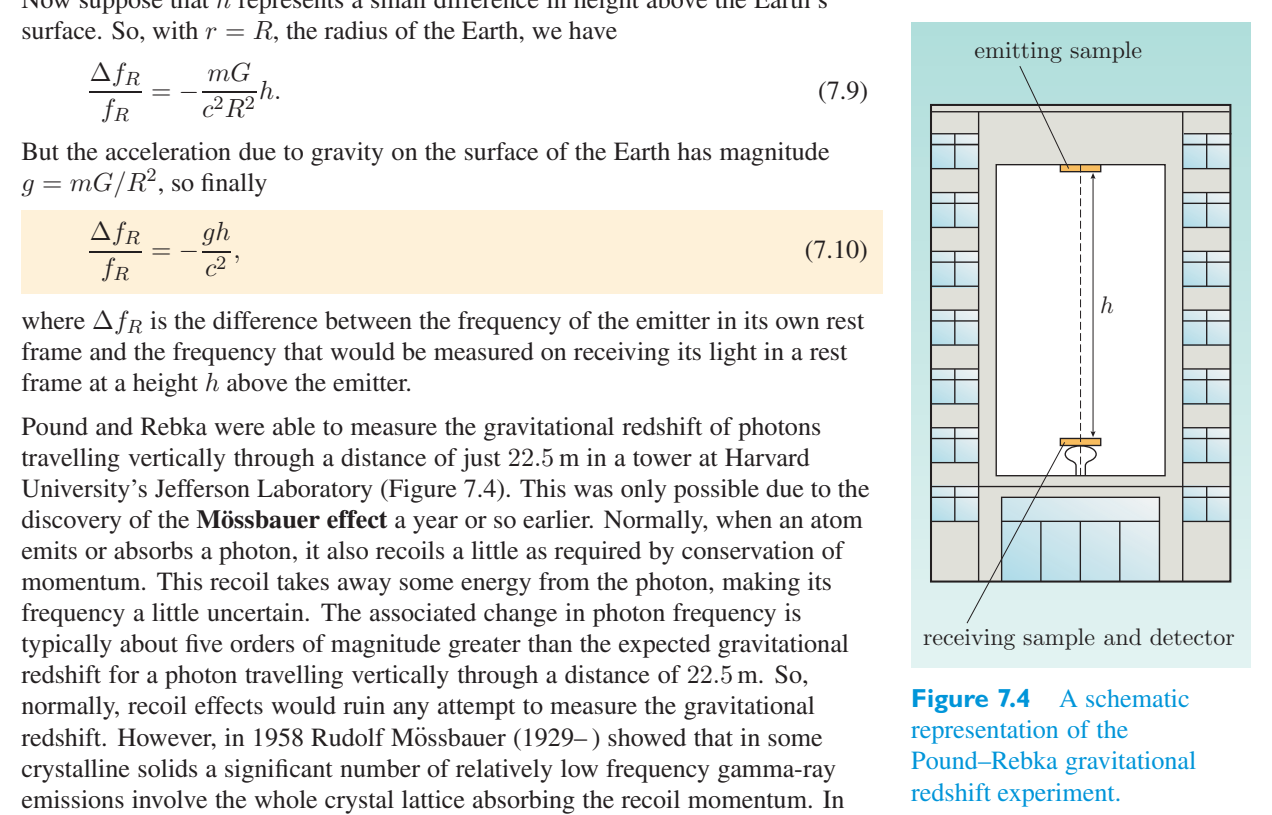
In the Pound–Rebka experiment, a solid sample containing Fe- 57, which emits 14 keV gamma rays, was placed in the centre of a loudspeaker cone near the top of the tower. By vibrating the loudspeaker cone, varying Doppler shifts were created in the photons emitted by the gamma-ray source. The Doppler-shifted gamma rays travelled vertically downwards through a Mylar bag filled with helium in order to minimize scattering of the gamma rays. Another sample containing Fe- 57 was placed in the basement, and a scintillation counter was placed below this in order to detect the gamma rays that were not absorbed by the receiving sample. When the Doppler shift imparted by the loudspeaker cancelled out the gravitational redshift, the receiving sample selectively absorbed the gamma rays, and the number of gamma rays detected by the scintillation counter dropped significantly. The variation in absorption could be correlated with the vibration frequency of the loudspeaker and hence with the Doppler shift and the gravitational redshift that it cancelled. This experiment by Pound and Rebka confirmed the gravitational redshift predictions of general relativity to about 10%, and this was later improved to better than 1% by Pound and Snyder.在 Pound-Rebka 实验中,含有 Fe-57 的固体样品(可发射 14 keV 伽马射线)被放置在靠近塔顶的扬声器锥体的中心。通过振动扬声器锥体,伽马射线源发射的光子会产生不同的多普勒频移。多普勒频移伽马射线垂直向下穿过充满氦气的聚酯薄膜袋,以最大限度地减少伽马射线的散射。另一个含有 Fe-57 的样品被放置在地下室中,闪烁计数器被放置在其下方,以检测未被接收样品吸收的伽马射线。当扬声器发出的多普勒频移抵消了引力红移时,接收样本选择性地吸收伽马射线,闪烁计数器检测到的伽马射线数量显着下降。吸收的变化可能与扬声器的振动频率相关,因此与多普勒频移及其抵消的引力红移相关。庞德和雷布卡的这个实验证实了广义相对论的引力红移预测达到了 10% 左右,后来庞德和斯奈德将这一结果改进到了 1% 以上。
Beyond the Pound–Rebka experiment超越英镑-雷布卡实验
In 1976, in an experiment known as Gravity Probe A, a hydrogen maser (a stable source of radiation with a very precise frequency) was briefly sent to a height of 10 km above the Earth, while its emissions were monitored from the ground. This experiment confirmed the predictions of gravitational time dilation to about 70 parts per million.1976 年,在一项名为引力探测器 A 的实验中,氢脉塞(具有非常精确频率的稳定辐射源)被短暂发送到距地球 10 公里的高度,同时从地面监测其发射。这个实验证实了引力时间膨胀约百万分之七十的预测。
An interesting application of gravitational time dilation is provided by the Global Positioning System (GPS). The GPS uses between 24 and 32 satellites that transmit precise microwave signals, enabling GPS receivers on or near the Earth’s surface to determine their location, speed, direction and time. Each satellite contains an atomic clock and orbits at about 20 200 km above the Earth’s surface. Since a satellite clock is in a weaker gravitational field than a ground-based one, it will tick more rapidly. Corrections are made for this effect by setting the satellite of 10.23 MHz. clock frequency to slightly less than the nominal frequency Because the functioning of the GPS is based on accurate timing, the effect of general relativity is significant, and if appropriate corrections were not made, errors in the positions of GPS receivers would accumulate at the rate of tens of kilometres per day. The continued accurate functioning of the GPS is therefore an experimental verification of general relativity. However, the accuracy of the verification (about 1%) is no better than for other experiments.全球定位系统(GPS)提供了引力时间膨胀的一个有趣的应用。 GPS 使用 24 到 32 颗卫星来传输精确的微波信号,使地球表面或附近的 GPS 接收器能够确定其位置、速度、方向和时间。每颗卫星都包含一个原子钟,并在距地球表面约 20 200 公里的轨道上运行。由于卫星时钟所处的引力场比地面时钟弱,因此它的走时速度会更快。通过将卫星设置为 10.23 MHz 来纠正这种影响。时钟频率略低于标称频率由于GPS的运行是建立在精确计时的基础上的,广义相对论的影响很大,如果不进行适当的修正,GPS接收机的位置误差将以每天数十公里的速度累积。因此,GPS 的持续精确运行是对广义相对论的实验验证。然而,验证的准确性(约 1%)并不比其他实验更好。
Exercise 7.3 (a) Calculate the time dilation due to练习 7.3 (a) 计算由于
general relativity for a GPS satellite clock compared to a ground-based clock.GPS 卫星时钟与地面时钟的广义相对论比较。
(b) Calculate the time dilation due to special relativity for a GPS satellite clock compared to a ground-based clock. (Ignore the satellite’s acceleration.)(b) 计算 GPS 卫星时钟与地面时钟相比由于狭义相对论而产生的时间膨胀。 (忽略卫星的加速度。)
(c) Estimate the error that results in a ground-based GPS receiver from the combined effect of (a) and (b).(c) 根据 (a) 和 (b) 的综合影响估计地面 GPS 接收器产生的误差。
7.1.4 Time delay of signals passing the Sun7.1.4 信号经过太阳的时间延迟
The three tests of general relativity that we have described so far could be described as the classic tests since they were proposed early in the history of the subject. However, a further classic test of general relativity, exploiting exceptionally high-powered radar, was proposed by Irwin I. Shapiro in 1964. The basic idea of the Shapiro time delay experiment is to record the transit times of radar signals from the Earth to a nearby planet (such as Mercury or Venus) and back. If the planet is just slipping around the back of the Sun (see path C–\(C'\) in Figure 7.5), then the radar pulse will probe the region close to the Sun where the spacetime metric differs most from that of special relativity. Since the orbit of the planet is well known from other astronomical observations, we can predict the travel times for all pulses going to and returning from the planet at any point in its orbit. If we made predictions assuming that spacetime is flat, we would find that they agree with experiment for all pulses except those that go close to the Sun’s edge. These pulses, which are probing the curved spacetime near to the Sun, take a slightly longer time than expected to come back.到目前为止,我们描述的广义相对论的三个检验可以说是经典检验,因为它们是在该学科历史的早期提出的。然而,欧文·夏皮罗 (Irwin I. Shapiro) 于 1964 年提出了广义相对论的进一步经典测试,即利用超高功率雷达。夏皮罗延时实验的基本思想是记录雷达信号从地球到附近行星(例如水星或金星)并返回的传输时间。如果行星只是绕太阳背面滑动(参见图 7.5 中的路径 C-\(C'\)),那么雷达脉冲将探测靠近太阳的区域,该区域的时空度规与狭义相对论的时空度规最大不同。由于行星的轨道通过其他天文观测是众所周知的,因此我们可以预测在其轨道上的任何点进出行星的所有脉冲的传播时间。如果我们假设时空是平坦的进行预测,我们会发现它们与所有脉冲的实验结果一致,除了那些靠近太阳边缘的脉冲。这些脉冲探测太阳附近的弯曲时空,返回的时间比预期稍长。
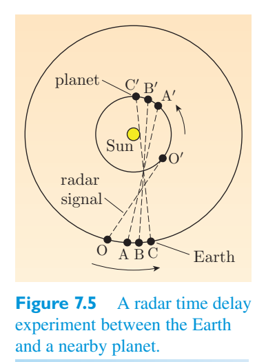
Using the Schwarzschild metric to represent the spacetime near the Sun, it can be shown that the total round-trip time for a radar pulse that travels from the Earth to the planet and back, with the pulse just grazing the Sun’s surface, is approximately given by使用史瓦西度规来表示太阳附近的时空,可以证明雷达脉冲从地球到行星再返回的总往返时间(脉冲刚刚掠过太阳表面)大约由下式给出
\(\Delta T\)(Earth–planet–Earth) ≈ \((R^2 - R^2)^{1/2}\) + \((R^2 - R^2)^{1/2}\)\(\Delta T\)(地球-行星-地球) ≈ \((R^2 - R^2)^{1/2}\) + \((R^2 - R^2)^{1/2}\)
where k is the Schwarzschild metric parameter (= G M)/\(c^2\) in this case) and R), R E and R P are the radial coordinates of the Sun’s surface, the Earth and the planet, respectively, as shown in Figure 7.6. The first thing to notice is what happens to this result if we set k equal to zero. This corresponds to saying that spacetime is everywhere like that of special relativity. The total travel time reduces in this case to其中 k 是史瓦西度规参数(在本例中 = G M)/\(c^2\)),R)、R E 和 R P 分别是太阳表面、地球和行星的径向坐标,如图 7.6 所示。首先要注意的是,如果我们将 k 设置为零,这个结果会发生什么。这相当于狭义相对论中时空无处不在的说法。在这种情况下,总行程时间减少为
This is just what we would expect; we would obtain precisely this result if we used Euclidean geometry to work out the total distance there and back (contained in the square bracket) and then divided the result by c to get the total travel time of the pulse. It is therefore the last term in curly brackets in Equation 7.11, multiplied by 4 k/c, that represents the effect of curved spacetime on \(\Delta T\).这正是我们所期望的;如果我们使用欧几里得几何计算出往返的总距离(包含在方括号中),然后将结果除以 c 以获得脉冲的总传播时间,我们将精确地获得此结果。因此,方程 7.11 中大括号中的最后一项乘以 4 k/c,代表弯曲时空对 \(\Delta T\) 的影响。
Equation 7.11 allows us to calculate the extra time delay due to the spacetime curvature. We know that light from the Sun takes about 8 minutes to get to the Earth. Thus the first term of Equation 7.11 will be of order 16 to 40 minutes, depending on the planet used. Now 4 k/c (= 4 G M)/\(c^3\)) is about 20 \(\mu\) s; so unless the term in the curly bracket is very large (which it won’t be — typical values are 10 to 15), the extra time delay predicted by general relativity is a tiny fraction of the total travel time. This illustrates the fact that general relativity predicts extremely small departures from Newton’s theory everywhere within the Solar System; there are simply no sufficiently large concentrations of mass within the Solar System for it to be otherwise.公式 7.11 允许我们计算由于时空曲率而产生的额外时间延迟。我们知道,来自太阳的光大约需要8分钟才能到达地球。因此,方程 7.11 的第一项约为 16 到 40 分钟,具体取决于所使用的行星。现在 4 k/c (= 4 G M)/\(c^3\)) 大约是 20 \(\mu\) s;因此,除非大括号中的项非常大(事实并非如此——典型值为 10 到 15),否则广义相对论预测的额外时间延迟只占总旅行时间的一小部分。这说明了一个事实,即广义相对论预测太阳系内各处与牛顿理论的偏差极小。太阳系内根本就没有足够大的质量集中度,因此不会出现这种情况。
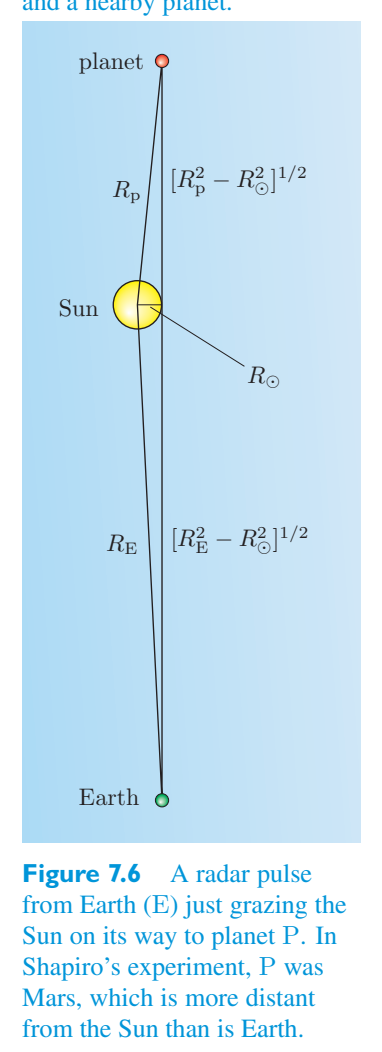
We can also see that the effect of the expression in the curly brackets of Equation 7.11 is to increase the time of travel of the pulse from that expected for the spacetime of special relativity; general relativity predicts a time delay. The quantity whose logarithm is to be taken can be written as我们还可以看到,方程 7.11 大括号中的表达式的效果是,相对于狭义相对论时空的预期,增加了脉冲的传播时间;广义相对论预言了时间延迟。要取对数的数量可以写为
Since自从
\(R'\) R and \(R'\) R,\(R'\) R 和 \(R'\) R,
we know that我们知道
and because natural logarithms of numbers greater than unity are positive, it follows that the whole term in curly brackets is positive.由于大于 1 的数字的自然对数是正数,因此大括号中的整个项都是正数。
Finally, we can put in some typical values of R E and R P, and the value of R), to get a quantitative estimate of the time delay caused by the effect of the Sun on the spacetime near it. At the outset of this calculation we should mention that the experimental problems involved in measuring radar pulse travel times are considerable, coming from a variety of sources, and we cannot do justice to the experiments here. A variation on Shapiro’s suggestion is to measure the time delay experienced by a signal transmitted by an artificial satellite or planetary probe as the signal passes close to the Sun. An example is given by experiments conducted during NASA’s Viking mission to Mars. This consisted of two space probes (launched in 1975) that orbited Mars, each equipped with a lander to study the planet from its surface. While one of the landers was on the surface of Mars, the time delay in a signal whose path was close to the Sun was measured. In this the Sun: \(2.254\times10^{11}\) m. case we must interpret R P as the distance of Mars from Putting this quantity along with R = \(1.496\times10^{11}\) m, R = \(6.960\times10^{8}\) m and 4 k/c = 4 G M/\(c^3\) = \(1.971\times10^{-5}\) s into the expression最后,我们可以代入一些典型的R E 和R P 值,以及R)的值,来定量估计太阳对其附近时空的影响所造成的时间延迟。在计算开始时,我们应该提到,测量雷达脉冲传播时间所涉及的实验问题相当多,来源多种多样,我们无法公正地对待这里的实验。夏皮罗建议的一个变体是测量人造卫星或行星探测器发射的信号在靠近太阳时所经历的时间延迟。美国宇航局维京号火星任务期间进行的实验就是一个例子。它由两个绕火星运行的太空探测器(1975 年发射)组成,每个探测器都配备了一个着陆器,可以从火星表面研究火星。当其中一个着陆器位于火星表面时,测量了路径靠近太阳的信号的时间延迟。在此太阳:\(2.254\times10^{11}\)米。在这种情况下,我们必须将 R P 解释为距火星的距离将此量与 R = \(1.496\times10^{11}\) m、R = \(6.960\times10^{8}\) m 和 4 k/c = 4 G M/\(c^3\) = \(1.971\times10^{-5}\) s 一起代入表达式
gives a predicted maximum time delay of 267 \(\mu\) s. The maximum delay observed in the Viking experiment was 250 \(\mu\) s; so our general relativistic calculation gives a reasonably accurate prediction of a time-delay effect of the Sun on a radio signal.给出了 267 \(\mu\) 秒的预测最大时间延迟。 Viking 实验中观察到的最大延迟为 250 \(\mu\) 秒;因此,我们的广义相对论计算可以相当准确地预测太阳对无线电信号的时滞效应。
Other space probes have subsequently been used in the measurement of the time delay experienced by a signal passing close to the Sun. NASA’s Voyager mission consisted of two probes, Voyagers 1 and 2, which were launched in 1977 with the aim of passing close to all the planets in the Solar System. The probes are still functioning and are now in the outer reaches of the Solar System. The time delay obtained using these probes is in agreement with the theoretical predictions with an accuracy of one part in one thousand. The Cassini probe was launched in 1997 with the aim of orbiting Saturn. In 2003, measurements on signals from the Cassini probe confirmed that the time delay agreed with the predictions of general relativity to about 20 parts in a million.其他空间探测器随后被用于测量靠近太阳的信号所经历的时间延迟。 NASA 的航行者号任务由两个探测器组成:航行者 1 号和航行者 2 号,它们于 1977 年发射,目的是靠近太阳系中的所有行星。探测器仍在运行,目前位于太阳系的外围。使用这些探头获得的时间延迟与理论预测一致,精度为千分之一。卡西尼号探测器于 1997 年发射,目标是环绕土星运行。 2003年,对卡西尼号探测器信号的测量证实,时间延迟与广义相对论的预测一致,约为百万分之二十。
This first section on classic tests of general relativity can be summarized as follows.关于广义相对论经典测试的第一部分可以总结如下。
Classic tests经典测试
The four classic tests of general relativity are as follows.广义相对论的四个经典检验如下。
1. The precession of the perihelion of Mercury The observations, which1. 水星近日点进动观测结果
have an uncertainty of about 1%, are consistent with the predictions of general relativity.不确定性约为1%,与广义相对论的预测一致。
2. Deflection of starlight by the Sun The observations, which have an2. 太阳对星光的偏转观测结果有
experimental uncertainty of about 10% for optical wavelengths, are in agreement with the predictions of general relativity. The agreement is better than 0.04% for VLBI radio telescope observations.光波长的实验不确定性约为 10%,与广义相对论的预测一致。 VLBI 射电望远镜观测结果的一致性优于 0.04%。
3. Gravitational redshift Gravitational redshift has been verified to better3. 引力红移引力红移已被验证可以更好地
than 1% in variants of the Pound–Rebka experiment. Gravity Probe A verified the time dilation due to general relativity to 70 parts per million. The continued functioning of the GPS confirms general relativistic time dilation to about 1% on a daily basis.在 Pound-Rebka 实验的变体中,这一比例低于 1%。引力探测器 A 验证了广义相对论引起的时间膨胀达到百万分之 70。 GPS 的持续运行证实了广义相对论时间每天膨胀约 1%。
4. Time delay of electromagnetic radiation passing the Sun The Cassini4. 卡西尼号电磁辐射穿过太阳的时间延迟
probe confirmed the effect to about 20 parts per million.探测器证实这种影响约为百万分之二十。
7.2 Satellite-based tests7.2 卫星测试
Soon after the formulation of general relativity, the Dutch astronomer Willem de Sitter (1872–1934) used Einstein’s theory to show that there would be a non-Newtonian contribution to the behaviour of the angular momentum of the Earth–Moon system as it orbited the Sun. The de Sitter effect, sometimes called the solar geodetic effect, is too small to provide a viable test of general relativity, but its discovery prompted others to consider more generally the way in which spinning bodies would transport angular momentum through curved spacetime. This led to predictions concerning the behaviour of orbiting gyroscopes that have recently been tested. This section first introduces the general relativistic phenomena involved in those tests and then discusses some of the results obtained.广义相对论提出后不久,荷兰天文学家威廉·德西特(Willem de Sitter,1872-1934)利用爱因斯坦的理论表明,地月系统绕太阳运行时的角动量行为将受到非牛顿贡献。德西特效应(有时称为太阳大地测量效应)太小,无法提供广义相对论的可行测试,但它的发现促使其他人更普遍地考虑旋转物体通过弯曲时空传输角动量的方式。这导致了对最近测试的轨道陀螺仪行为的预测。本节首先介绍这些测试中涉及的广义相对论现象,然后讨论获得的一些结果。
7.2.1 Geodesic gyroscope precession7.2.1 测地陀螺进动
A gyroscope is a device that uses the angular momentum of a spinning body to indicate a particular direction in space. Gyroscope designs vary, but a common sort consists of a heavy rotatable disc mounted in a set of very low friction bearings that allow the disc’s axis of rotation to point in any direction (Figure 7.7). The disc is symmetric, so when it is made to spin rapidly, its angular momentum is aligned with the axis of rotation. In a flat spacetime the whole gyroscope can be moved without altering the angular momentum of the disc, so the axis of rotation will indicate a fixed direction in space. This principle is used as the basis of the gyrocompass, which has many applications in air and sea navigation.陀螺仪是一种利用旋转体的角动量来指示空间中特定方向的装置。陀螺仪的设计各不相同,但常见的一种是由安装在一组摩擦力极低的轴承中的重型旋转盘组成,允许盘的旋转轴指向任何方向(图 7.7)。圆盘是对称的,因此当它快速旋转时,其角动量与旋转轴对齐。在平坦的时空中,整个陀螺仪可以在不改变圆盘角动量的情况下移动,因此旋转轴将指示空间中的固定方向。这一原理被用作陀螺罗盘的基础,在空中和海上导航中有许多应用。
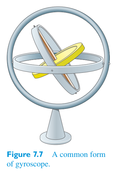
In a region where spacetime is curved, the situation is rather different. In curved spacetime, the centre of mass of a freely falling gyroscope will move along a geodesic, and the angular momentum of the gyroscope will be transported along that geodesic. We saw earlier that the four-velocity of a freely falling particle is parallel transported along the geodesic that the particle follows, and in a similar way the angular momentum associated with the spin of a freely falling gyroscope will also be parallel transported along the geodesic. Even so, the presence of curvature will generally cause the direction of the spin angular momentum to change. (You saw in Chapter 3 that when a vector is parallel transported around a closed loop, the orientation of that vector changes in a way that depends on the spacetime curvature.)在时空弯曲的区域,情况则截然不同。在弯曲时空中,自由落体陀螺仪的质心将沿着测地线移动,陀螺仪的角动量将沿着该测地线传输。我们之前看到,自由落体粒子的四速度沿着粒子所遵循的测地线平行传输,类似地,与自由落体陀螺仪自旋相关的角动量也将沿着测地线平行传输。即便如此,曲率的存在通常会导致自旋角动量的方向发生变化。(您在第 3 章中看到,当矢量绕闭环平行传输时,该矢量的方向会以取决于时空曲率的方式发生变化。)
As a comparatively straightforward example, consider a gyroscope moving in free fall around a spherically symmetric body of mass M. Suppose that the gyroscope is in a polar orbit of radius r, and that initially the spin angular momentum vector of the gyroscope points radially away from the centre of the massive body. In a flat spacetime we know that after one complete orbit the angular momentum vector will remain radial and that this will still be true after any number of orbits. However, according to general relativity the spacetime in the vicinity of the gyroscope is not flat but can be described by the Schwarzschild metric. Using this metric, it can be shown that after one orbit the angular momentum vector of the gyroscope is no longer radial but will have precessed by a small angle \(\alpha\) in the plane of the orbit, as shown in Figure 7.8. The precession作为一个相对简单的例子,考虑一个围绕质量为 M 的球对称体自由落体运动的陀螺仪。假设陀螺仪位于半径为 r 的极轨道上,并且最初陀螺仪的自旋角动量矢量径向远离质量体的中心。在平坦的时空中,我们知道,在一个完整的轨道之后,角动量矢量将保持径向,并且在任意数量的轨道之后,这仍然是正确的。然而,根据广义相对论,陀螺仪附近的时空并不平坦,但可以用史瓦西度规来描述。使用这个度规可以表明,在绕一圈之后,陀螺仪的角动量矢量不再是径向的,而是在轨道平面上进动了一个小角度 \(\alpha\),如图 7.8 所示。进动
This effect is sometimes known as geodesic gyroscope precession, though it is also often referred to as the geodetic effect. It is a very small effect, but since it is cumulative, it can become significant over many orbits.这种效应有时被称为测地陀螺仪进动,尽管它也经常被称为大地测量效应。这是一个非常小的影响,但由于它是累积的,因此在许多轨道上它会变得很重要。
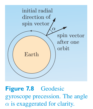
Exercise 7.4 Confirm that for a gyroscope with angular练习 7.4 确认对于具有角度的陀螺仪
momentum vector initially radial, in a low Earth orbit, the precession is about \(8''\) per year.动量矢量最初是径向的,在近地轨道上,进动约为每年 \(8''\)。
7.2.2 Frame dragging7.2.2 框拖动
In the neighbourhood of a rotating body, such as a rotating black hole, spacetime is more accurately described by the axially symmetric Kerr metric rather than the spherically symmetric Schwarzschild metric. As you saw earlier, the Kerr metric implies the dragging of inertial frames around the rotating body. This too can give rise to gyroscopic precession, though it is quite distinct from the geodesic precession described in the previous section.在旋转体(例如旋转黑洞)的附近,时空可以通过轴对称克尔度规而不是球对称史瓦西度规更准确地描述。正如您之前所看到的,克尔度规意味着围绕旋转体拖动惯性系。这也可能引起陀螺进动,尽管它与上一节中描述的测地线进动截然不同。
The rotational dragging of inertial frames is sometimes referred to as the Lense–Thirring effect after Josef Lense (1890–1985) and Hans Thirring (1888–1976), the scientists who deduced the existence of such an effect in 1918, long before the introduction of the Kerr metric. In fact, the rotational dragging of inertial frames is a particular case of a more general phenomenon of frame dragging that takes place whenever there is a significant movement of matter (a mass current) in the neighbourhood of a locally inertial frame.惯性系的旋转拖动有时被称为 Lense-Thirring 效应,这是由 Josef Lense(1890-1985)和 Hans Thirring(1888-1976)这两位科学家在 1918 年(早在克尔度规引入之前很久)就推断出这种效应存在的。事实上,惯性系的旋转拖动是更普遍的坐标系拖动现象的一个特例,每当局部惯性系附近存在显着的物质运动(质量流)时就会发生这种现象。
For a slowly rotating body, such as the Earth, the Lense–Thirring effect is very small and difficult to observe. One way to understand the consequences of frame dragging is to consider a satellite in a polar orbit about the Earth. If the Earth was isolated, perfectly symmetric, and didn’t rotate, then the plane of the satellite’s orbit would remain fixed. However, since the Earth does in fact rotate about an axis through the poles, frame dragging predicts that the plane of the satellite’s orbit will rotate very slowly in the same direction as the Earth’s rotation, as indicated in Figure 7.9. An effect of frame dragging is to induce a very small precession in a gyroscope orbiting the Earth. If the rotation axis of the gyroscope is initially in the equatorial plane of the planet and points radially away from the planet’s centre, then the Lense–Thirring effect will cause the spin axis to precess eastward but the rate will be less than 1% of that due to geodesic precession.对于缓慢旋转的物体,例如地球,透镜-蒂林效应非常小且难以观察。了解坐标系拖动后果的一种方法是考虑一颗绕地球极地轨道运行的卫星。如果地球是孤立的、完全对称的并且不旋转,那么卫星轨道平面将保持固定。然而,由于地球实际上确实绕着穿过两极的轴旋转,因此参考系拖动预测卫星轨道平面将沿着与地球自转相同的方向非常缓慢地旋转,如图 7.9 所示。参考系拖动的一个效果是在绕地球运行的陀螺仪中引起非常小的进动。如果陀螺仪的旋转轴最初位于行星的赤道平面上,并径向远离行星中心,则 Lense-Thirring 效应将导致自转轴向东进动,但进动速率将小于测地进动造成的进动速率的 1%。
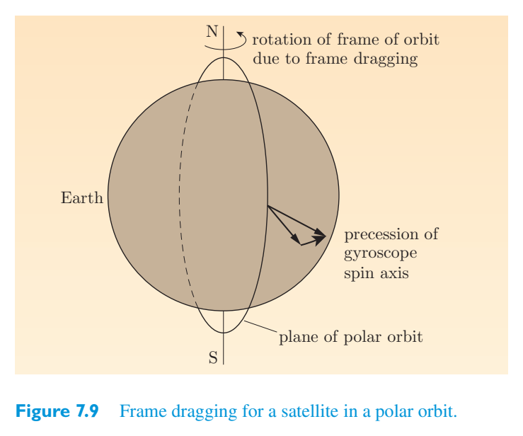
7.2.3 The LAGEOS satellites7.2.3 LAGEOS 卫星
The satellites LAGEOS I (launched in 1976) and LAGEOS II (launched in 1992) are simply heavy (411 kg) spheres, 60 cm in diameter, that orbit at a height of 5900 km above the Earth’s surface. They have no on-board electronics, but are covered in retro-reflectors, which are used for laser ranging from ground tracking stations. One of the satellites is shown in Figure 7.10.LAGEOS I(1976 年发射)和 LAGEOS II(1992 年发射)卫星是直径 60 厘米、重(411 公斤)的球体,在距地球表面 5900 公里的高度运行。它们没有机载电子设备,但覆盖有后向反射器,用于地面跟踪站的激光测距。其中一颗卫星如图 7.10 所示。
The satellites enable very accurate measurements to be made of their positions relative to points on the Earth’s surface. Such observations have been used to produce an accurate picture of how the Earth’s gravitational field differs from that produced by a uniform sphere, and to make precise measurements of continental drift. One research group claims that the plane of the orbits of the LAGEOS I and II satellites appears to be shifting, confirming the frame dragging prediction of general relativity to better than 10%. However, the result is highly controversial because other estimates of the probable error are very much higher than 10%. The most common view amongst experts in the field is that the LAGEOS results are interesting but inconclusive. They do not call general relativity into question, but nor do they provide any meaningful confirmation of the theory.这些卫星能够非常精确地测量它们相对于地球表面点的位置。这些观测已被用来准确描述地球引力场与均匀球体产生的引力场的不同,并精确测量大陆漂移。一个研究小组声称,LAGEOS I 和 II 卫星的轨道平面似乎正在发生移动,证实了广义相对论的参考系拖拽预测优于 10%。然而,这一结果颇具争议,因为其他估计的可能误差远高于 10%。该领域专家最普遍的观点是,LAGEOS 的结果很有趣,但尚无定论。他们没有对广义相对论提出质疑,但也没有对该理论提供任何有意义的证实。
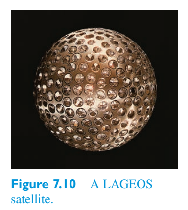
7.2.4 Gravity Probe B7.2.4 引力探针B
Gravity Probe B was an ambitious project using cutting edge technology to test general relativity. It was based on a polar orbiting satellite that was launched in April 2004 to a height of 642 km above the Earth.引力探测器 B 是一个雄心勃勃的项目,利用尖端技术来测试广义相对论。它是基于一颗极轨卫星,于 2004 年 4 月发射到距地球 642 公里的高度。
To give a greatly simplified description of the experiment, the satellite contained a telescope and a set of four gyroscopes (four were used to increase the sensitivity and provide redundancy). Each gyroscope took the form of an electrically levitated sphere made from fused quartz coated with a thin layer of niobium. At the time of their production, the gyroscopes were the most perfect spherical objects ever constructed. The gyroscopes and their housings were contained within lead shields, and the whole assembly was cooled to a few degrees above absolute zero so that the niobium and the lead were superconducting. The superconductivity ensured that external electromagnetic fields were screened out and played an important part in enabling the rotation axis of each gyroscope to be accurately monitored without disturbing the rotation.为了大大简化实验的描述,卫星包含一个望远镜和一组四个陀螺仪(四个用于提高灵敏度并提供冗余)。每个陀螺仪均采用电悬浮球体的形式,由涂有一层薄薄铌的熔融石英制成。在生产时,陀螺仪是有史以来最完美的球形物体。陀螺仪及其外壳包含在铅屏蔽内,整个组件被冷却到绝对零以上几度,以便铌和铅具有超导性。超导性确保了外部电磁场被屏蔽,并在不干扰旋转的情况下准确监测每个陀螺仪的旋转轴方面发挥了重要作用。
At the start of the experiment, the telescope and gyroscopes were aligned with a guide star and the telescope was kept aligned with that guide star for 50 weeks, during which time the satellite continued in its polar orbit. The idea was to measure the change in the spin axis alignment of each gyroscope over the 50 weeks (a) in the plane of the orbit and (b) in the Earth’s equatorial plane, as shown in Figure 7.11. Result (a) indicates the geodesic precession, predicted by general relativity to be 6.606 arcseconds (0.0018 ◦) per year. Gravity Probe B was expected to test this result to an accuracy of 0.01%. Result (b) is the frame dragging precession due to the Lense–Thirring effect and had not previously been measured. Gravity Probe B was expected to test this result to an accuracy of 1%.实验开始时,望远镜和陀螺仪与一颗导星对齐,并且望远镜与该导星保持对齐 50 周,在此期间卫星继续在极地轨道上运行。这个想法是测量每个陀螺仪自旋轴对准在 50 周内的变化(a)在轨道平面上和(b)在地球赤道平面上,如图 7.11 所示。结果 (a) 表明测地进动,根据广义相对论预测为每年 6.606 角秒 (0.0018 °)。引力探测器 B 预计将测试该结果,准确度为 0.01%。结果 (b) 是由 Lense-Thirring 效应引起的参考系拖曳进动,之前未曾测量过。引力探测器 B 预计将测试该结果,准确度为 1%。
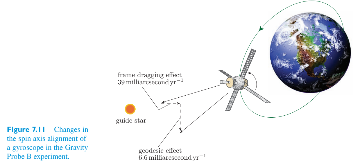
The results so far are that (a) the experiment has confirmed the geodesic precession effect to 1.5%, but (b) the expected frame dragging is below the noise level of the data. This noise is due to unexpected torques on the gyroscopes, which the project team is currently trying to model.到目前为止的结果是:(a) 实验已确认测地线进动效应为 1.5%,但 (b) 预期的帧拖动低于数据的噪声水平。这种噪音是由于陀螺仪上的意外扭矩造成的,项目团队目前正在尝试对其进行建模。
We summarize the results of this section as follows.我们将本节的结果总结如下。
Satellite-based tests基于卫星的测试
Satellite-based tests aim to detect two effects:基于卫星的测试旨在检测两种效果:
- • geodesic gyroscope precession• 测地陀螺进动
- • rotational frame dragging (Lense–Thirring effect).• 旋转框架拖动(Lense–Thirring 效果)。
Two satellite-based tests are:两项基于卫星的测试是:
1. The LAGEOS satellite results, which have been claimed to confirm frame1. LAGEOS卫星结果,据称证实了帧
dragging to 10%, but this is disputed.拖到10%,但这是有争议的。
2. Gravity Probe B results, which confirm geodesic gyroscope precession to2. 引力探测器 B 结果,证实了测地陀螺仪进动
1.5%. The expected frame dragging is below the noise level, though there is1.5%。预期的帧拖动低于噪声水平,尽管存在
still some hope that further analysis might improve the situation.仍有一些人希望进一步的分析可以改善这种情况。
Exercise 7.5 Calculate the expected geodesic precession per year for a练习 7.5 计算每年预期的测地进动
gyroscope in the Gravity Probe B experiment.引力探测器 B 实验中的陀螺仪。
7.3 Astronomical observations7.3 天文观测
This section concerns astronomical observations of gravitational lenses and systems believed to contain black holes. Neither kind of observation provides a direct test of general relativity, but each concerns non-Newtonian behaviour and contributes to the body of circumstantial evidence that supports general relativity. There is an important additional strand of evidence that comes from observations of pulsars (rotating magnetic neutron stars), but this is considered separately in the next section.本节涉及对被认为包含黑洞的引力透镜和系统的天文观测。这两种观察都没有提供对广义相对论的直接检验,但每一种都涉及非牛顿行为,并为支持广义相对论提供了间接证据。还有一条重要的额外证据来自对脉冲星(旋转磁中子星)的观测,但这将在下一节中单独考虑。
7.3.1 Black holes7.3.1 黑洞
Black holes were discussed at length in Chapter 6. There, they were mainly treated as idealized classical spacetime structures in which a singularity is contained within an event horizon. It was suggested that such singularities might arise from the catastrophic gravitational collapse of stars that had exhausted their core nuclear fuel and were too massive to exist stably as white dwarfs or neutron stars. It was pointed out that quantum effects might prevent the formation of singularities, but no mechanism for this is currently known, and even if it happened, it would not preclude the existence of bodies that are essentially indistinguishable from black holes. Once a black hole is formed, its mass can increase due to the capture of stars, interstellar matter or other black holes.黑洞在第六章中进行了详细讨论。在那里,它们主要被视为理想化的经典时空结构,其中奇点包含在事件视界内。有人认为,这种奇点可能是由恒星的灾难性引力塌缩引起的,这些恒星已经耗尽了核心核燃料,并且质量太大,无法以白矮星或中子星的形式稳定存在。有人指出,量子效应可能会阻止奇点的形成,但目前尚不清楚这种机制,即使它发生了,也不会排除与黑洞本质上没有区别的物体的存在。黑洞一旦形成,其质量就会因恒星、星际物质或其他黑洞的捕获而增加。
Evidence concerning black holes is most easily organized by considering in turn the various mass regimes: mini, stellar, intermediate and supermassive.有关黑洞的证据最容易通过依次考虑各种质量状态来组织:微型、恒星、中等质量和超大质量。
Mini black holes迷你黑洞
Black holes with masses in the range 0 M) to 0.1 M) (where M) is the mass of the Sun) have not been observed. Very low mass black holes will be sought in the high-energy proton collisions at the Large Hadron Collider in CERN. Higher mass mini black holes have already been sought astronomically but without success. This is not altogether surprising since there is no obvious route for their production, though they might have been formed in the early Universe. As we saw in Chapter 6, evaporating mini black holes are expected to emit Hawking radiation and should end their lives in an explosion. Such explosions could release detectable amounts of gamma radiation. Astronomical sources of gamma-ray bursts have been detected, but their properties are different from those expected of an exploding mini black hole so the two phenomena are currently thought to be unrelated. The Hawking radiation from any mini black holes that do exist will contribute gamma rays and particles such as antiprotons to the cosmic radiation that reaches the Earth from space. Studies of the composition of cosmic rays not only fail to give direct evidence of mini black holes, but also impose limits on the abundance of mini black holes in the Universe.尚未观测到质量在 0 M) 至 0.1 M) 范围内的黑洞(其中 M)是太阳的质量)。欧洲核子研究中心大型强子对撞机的高能质子对撞将寻找极低质量黑洞。天文学上已经开始寻找更高质量的迷你黑洞,但没有成功。这并不完全令人惊讶,因为它们的产生没有明显的途径,尽管它们可能是在早期宇宙中形成的。正如我们在第六章中看到的,蒸发的微型黑洞预计会发出霍金辐射,并会以爆炸结束它们的生命。此类爆炸可能会释放出可检测量的伽马辐射。伽马射线暴的天文来源已经被发现,但它们的特性与预期的微型黑洞爆炸的特性不同,因此目前认为这两种现象是无关的。来自任何确实存在的微型黑洞的霍金辐射都会向从太空到达地球的宇宙辐射贡献伽马射线和反质子等粒子。对宇宙射线成分的研究不仅无法给出微型黑洞存在的直接证据,而且还限制了宇宙中微型黑洞的丰度。
Stellar mass black holes恒星质量黑洞
Black holes with masses in the range of a few M) to a few tens of M) are such feeble sources of Hawking radiation that, for all practical purposes, they are truly ‘black’ and therefore not directly observable. Nonetheless, substantial indirect evidence of their existence has been (and continues to be) accumulated. This evidence comes mainly from the study of binary star systems in which the supposed black hole is detected via its interaction with a companion star. The components of a binary system can sometimes be sufficiently close together that material from the atmosphere of a star is transferred to the companion body. The transfer is particularly easy if the donor star is a giant or a supergiant with an enormously distended atmosphere and a significant stellar wind, or if the two stars are close enough together for the donor star to fill its Roche lobe. (The Roche lobe is the teardrop-shaped region around a star where the gravitational effect of the star is stronger than that due to its binary companion.) Either method of mass transfer can lead to the emission of X-rays if the receiving body is a compact object, such as a black hole, a neutron star or possibly a white dwarf. The transferred material is quite likely to have too much angular momentum to fall directly onto the compact object. If so, it will form a rotating disc around the compact object. The study of these discs has become an important topic in astrophysics and is discussed in detail in this book’s companion volume, Extreme Environment Astrophysics by Ulrich Kolb.质量在几M到几十M范围内的黑洞是非常微弱的霍金辐射源,出于所有实际目的,它们是真正的“黑色”,因此无法直接观测到。尽管如此,关于它们存在的大量间接证据已经(并将继续)积累起来。这一证据主要来自对双星系统的研究,在双星系统中,所谓的黑洞是通过其与伴星的相互作用而被检测到的。双星系统的组成部分有时可能足够接近,以至于来自恒星大气层的物质会转移到伴星上。如果供体恒星是一颗巨星或超巨星,具有极大膨胀的大气层和显着的星风,或者如果两颗恒星距离足够近,供体恒星可以填满其洛希瓣,那么转移就特别容易。(罗氏瓣是恒星周围的泪滴状区域,其中恒星的引力效应比其双星伴星的引力效应更强。)如果接收体是致密天体,例如黑洞、中子星或可能是白矮星,则任何一种质量传递方法都可以导致 X 射线的发射。转移的材料很可能具有太大的角动量而无法直接落在致密物体上。如果是这样,它将在致密物体周围形成一个旋转圆盘。对这些圆盘的研究已成为天体物理学的一个重要课题,并在本书的姊妹篇乌尔里希·科尔布(Ulrich Kolb)的《极端环境天体物理学》中进行了详细讨论。
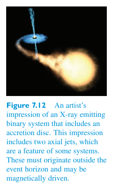
The material in a rotating disc encircling a black hole is subject to tidal effects and to friction. These will heat the disc material and cause it to spiral inwards to the point where it can be accreted by the compact body. It is for this reason that these discs are usually referred to as accretion discs. The heating of the in-falling matter is such that it can emit X-rays, making the system a suitable target for detection by astronomers working at X-ray wavelengths. Many X-ray emitting binary systems are now known, and an artist’s impression of such a system is given in Figure 7.12.环绕黑洞的旋转圆盘中的物质会受到潮汐效应和摩擦力的影响。这些将加热圆盘材料并使其向内螺旋至可以被致密体吸积的点。正是由于这个原因,这些盘通常被称为吸积盘。坠落物质的加热使其能够发射 X 射线,使该系统成为天文学家在 X 射线波长下进行探测的合适目标。现在已知许多发射 X 射线的双星系统,图 7.12 给出了这种系统的艺术印象。
The task of the black hole hunter is to distinguish those systems in which the compact object must be a black hole from those in which it might be a neutron star or a white dwarf. This is done on the basis of the compact object’s mass. It is known that there is an upper limit to the mass of a white dwarf (the Chandrasekhar limit, about 1.4 M)) and also an upper limit to the mass of a neutron star (the Oppenheimer–Volkoff limit, about 2.5 M)). Consequently, an X-ray emitting binary system in which there is a compact partner that can be shown to have a mass that exceeds the Oppenheimer–Volkoff limit is regarded as containing a black hole. The Oppenheimer–Volkoff limit is not particularly well determined so, generally speaking, the greater the mass of the candidate, the better the case for believing it to be a black hole. Unfortunately, the mass determination is rarely straightforward. It is usually based on observations of Doppler shifts in the frequency of the radiation emitted by the system and can be subject to uncertainty arising from the inclination of the compact body’s orbit.黑洞猎人的任务是将致密天体必须是黑洞的系统与可能是中子星或白矮星的系统区分开来。这是根据致密物体的质量来完成的。众所周知,白矮星的质量有上限(钱德拉塞卡极限,约1.4 M)),中子星的质量也有上限(奥本海默-沃尔科夫极限,约2.5 M))。因此,一个发射 X 射线的双星系统,如果其中有一个质量超过奥本海默-沃尔科夫极限的致密伙伴,则被视为包含黑洞。奥本海默-沃尔科夫极限并不是特别确定,因此,一般来说,候选者的质量越大,就越有可能相信它是黑洞。不幸的是,质量测定很少是直接的。它通常基于对系统发射的辐射频率的多普勒频移的观测,并且可能受到致密体轨道倾斜引起的不确定性的影响。
One well-known stellar mass black hole candidate is Cygnus X-1, the strongest X-ray source in the constellation of Cygnus. It was first detected in 1964, in the early days of X-ray astronomy, using a rocket-borne detector. Later studies confirmed it as an intense source of X-rays but also showed that it was a highly irregular variable source. Its shortest fluctuations are on timescales of milliseconds, implying that the X-ray emitting region is unlikely to be more than about a millilightsecond across (300 km), which is just what might be expected of a gravitationally collapsed star and the inner part of an accretion disc. In the early 1970s, when the position of Cygnus X-1 was accurately determined for the first time, it was found to be associated with the blue supergiant star HDE 226868. Periodically varying Doppler shifts in the spectral lines of that star indicate that it is part of a binary system with a 5.6 -day orbital period. The amplitude of the variations in Doppler shift provides further information about the orbit, and together with the period strongly suggests that the compact companion has a mass that is greater than 4.8 M). Additional arguments concerning the system’s distance and its lack of eclipses suggest that the mass of the compact component is actually well above this minimum, probably in the range 7 – 13 M). All this makes it very likely that Cygnus X-1 consists of a black hole with an accretion disc that is supplied with matter by HDE 226868. About 20 broadly similar stellar mass black hole systems are currently known, with a further 20 or so candidate systems, representing a range of black hole and companion star masses.天鹅座 X-1 是一个著名的恒星质量黑洞候选者,它是天鹅座中最强的 X 射线源。它于 1964 年首次被探测到,当时正值 X 射线天文学的早期阶段,使用的是火箭载探测器。后来的研究证实它是一个强烈的 X 射线源,但也表明它是一个高度不规则的可变源。它的最短波动是在毫秒的时间尺度上,这意味着X射线发射区域的宽度不太可能超过约一毫秒(300公里),这正是对引力塌缩恒星和吸积盘内部的预期。20世纪70年代初,当天鹅座X-1的位置首次被精确确定时,人们发现它与蓝色超巨星HDE 226868有关。该恒星谱线中周期性变化的多普勒频移表明它是轨道周期为5.6天的双星系统的一部分。多普勒频移变化的幅度提供了有关轨道的进一步信息,并且与周期一起强烈表明紧凑伴星的质量大于 4.8 M)。关于系统距离及其缺乏日食的其他论点表明,紧凑组件的质量实际上远高于此最小值,可能在 7 – 13 M 范围内。所有这些使得天鹅座 X-1 很可能由一个带有吸积盘的黑洞组成,吸积盘由 HDE 226868 提供物质。目前已知大约 20 个大致相似的恒星质量黑洞系统,还有另外 20 个左右的候选系统,代表了一系列黑洞和伴星质量。
The evidence that some X-ray emitting binaries contain a compact object that is too massive to be a neutron star is strong. But the additional step of saying that this object is a black hole is based on the lack of any credible alternative; there is no direct evidence of an ev ent horizon or any other feature that might be considered specific to general relativity. However, indirect evidence that an event horizon is present can be obtained from the observed variations in the intensity of X-rays emitted by such binary systems. Much of this variation is attributed to changes in the rate at which matter is being supplied to the central compact object via the accretion disc. When the X-ray intensity is low, it is presumed that the rate of in-fall is small — perhaps little more than a trickle. Under these circumstances material falling onto a neutron star would continue to contribute to the total intensity of the source as long as it was hot, but material falling into a black hole would be lost from sight as it dimmed rapidly when approaching the event horizon. If the observed X-ray emitting binaries are divided into two classes according to whether the compact object has a mass below 2 M) or above 3 M), it is found that the former objects have a higher minimum X-ray intensity than the latter. This has been interpreted as evidence that in the latter case, where the compact object has a mass that is above the Oppenheimer–Volkoff limit, an event horizon is indeed present. We shall have more to say about X-ray evidence later.有强有力的证据表明,一些发射 X 射线的双星包含一个质量太大而无法成为中子星的致密天体。但说这个物体是黑洞的额外步骤是基于缺乏任何可信的替代方案;没有直接证据表明事件视界或任何其他可能被认为是广义相对论特有的特征。然而,可以从观测到的此类双星系统发射的 X 射线强度的变化中获得事件视界存在的间接证据。这种变化很大程度上归因于通过吸积盘向中心致密天体提供物质的速率的变化。当 X 射线强度较低时,人们推测坠落的速度很小——也许只是涓涓细流。在这种情况下,只要落入中子星的物质很热,落入中子星的物质就会继续对源的总强度做出贡献,但落入黑洞的物质会在接近视界时迅速变暗,从而从视线中消失。如果将观测到的发射X射线的双星根据致密天体的质量是小于2M)还是大于3M)分为两类,则发现前者的最小X射线强度高于后者。这被解释为证明在后一种情况下,当致密物体的质量高于奥本海默-沃尔科夫极限时,事件视界确实存在。稍后我们将更多地讨论 X 射线证据。
In addition to the evidence from close binary systems, there is additional evidence for stellar mass black holes from a process known as gravitational microlensing. This is sensitive to isolated black holes as well as those in binary systems. It will be mentioned again when we discuss gravitational lensing in the next section.除了来自紧密双星系统的证据之外,还有来自称为引力微透镜的过程的恒星质量黑洞的额外证据。这对孤立的黑洞以及双星系统中的黑洞很敏感。我们在下一节讨论引力透镜时会再次提到这一点。
Intermediate mass black holes中等质量黑洞
Black holes with masses in the range 100 M) to 10 5 M) have been sought for many years. It is probably fair to say that there is growing evidence that they may exist in various clusters of stars both within the Milky Way and in some external galaxies. However, there are still many astronomers who doubt the existence of black holes in this class, especially because it is not clear how they would form. Since their existence is still in doubt both theoretically and observationally, intermediate black holes cannot currently be said to provide any sort of test of general relativity.多年来,人们一直在寻找质量在 100 M) 至 10 5 M) 范围内的黑洞。可以公平地说,越来越多的证据表明它们可能存在于银河系内和一些外部星系的各种星团中。然而,仍然有许多天文学家怀疑此类黑洞的存在,特别是因为尚不清楚它们是如何形成的。由于它们的存在在理论上和观测上仍然存在疑问,因此目前不能说中间黑洞提供了任何形式的广义相对论测试。
Supermassive black holes超大质量黑洞
Black holes with masses in excess of 10 5 M) are not only thought to exist, but are believed to be common. The most direct evidence for their existence comes from studying the behaviour of stars and gas clouds close to the centres of galaxies. In the case of our own galaxy, the Milky Way, extensive studies of this kind, based on observations of stellar orbits at infrared wavelengths, have provided of about \(2.5\times10^{6}\) M), strong evidence of a compact central object with a mass contained within a volume comparable to that of the inner Solar System. This object is associated with Sagittarius A* (pronounced A-star), a strong radio source located at the centre of the Milky Way. Another example is at the centre of the galaxy NGC 4258, which has been observed using very long baseline interferometry (VLBI). The results show clear evidence of a compact object with a mass of \(4\times10^{7}\) M). Many other examples are known, and there is growing evidence that each of these central objects has a mass that is directly related to the mass of the spheroidal component of its host galaxy. This correlation suggests that the formation of galactic centre black holes may be a natural part of the process of galaxy formation rather than something that happens by accident in a few galaxies.质量超过 10 5 M 的黑洞不仅被认为存在,而且被认为很常见。它们存在的最直接证据来自于研究靠近星系中心的恒星和气体云的行为。就我们自己的星系银河系而言,基于对红外波长恒星轨道的观测,进行了广泛的此类研究,提供了大约 \(2.5\times10^{6}\) M) 的有力证据,证明存在一个紧凑的中心天体,其质量与内太阳系的体积相当。该天体与人马座 A*(发音为 A-star)有关,人马座 A* 是位于银河系中心的强射电源。另一个例子位于 NGC 4258 星系的中心,人们使用甚长基线干涉仪 (VLBI) 对其进行了观测。结果清楚地表明存在一个质量为 \(4\times10^{7}\) M) 的致密天体。许多其他例子是已知的,并且越来越多的证据表明,每个中心天体的质量都与其宿主星系的球体成分的质量直接相关。这种相关性表明,星系中心黑洞的形成可能是星系形成过程的自然组成部分,而不是少数星系中偶然发生的事情。
\(2.5\times10^{6}\) M) and\(2.5\times10^{6}\) M) 和
- ● What are the Schwarzschild radii corresponding to● 史瓦西半径对应于什么
\(4\times10^{7}\) M?\(4\times10^{7}\) M?
❍ The Schwarzschild radius R = 2 GM/\(c^2\) corresponding to 1 M is 3 km. so \(2.5\times10^{6}\) M) The Schwarzschild radius grows in proportion to mass, corresponds to \(7.5\times10^{6}\) km, and \(4\times10^{7}\) M corresponds to \(12\times10^{7}\) km.❍ 史瓦西半径 R = 2 GM/\(c^2\) 对应 1 M 为 3 km。所以 \(2.5\times10^{6}\) M) 史瓦西半径与质量成比例增长,对应于 \(7.5\times10^{6}\) km,\(4\times10^{7}\) M 对应于 \(12\times10^{7}\) km。
Dynamical studies of stars and gas clouds close to galactic centres give evidence of compact massive bodies but they do not prove that those bodies really are black holes. However, this issue is addressed to some extent by detailed studies of X-ray spectra.对靠近银河系中心的恒星和气体云的动力学研究提供了致密大质量天体的证据,但并不能证明这些天体确实是黑洞。然而,通过对 X 射线光谱的详细研究,这个问题在一定程度上得到了解决。
Figure 7.13 shows a distorted spectral line seen in the X-ray spectrum of the galaxy MCG-6-30-15. This feature is believed to be due to ionized iron atoms that travel around the galaxy’s central black hole as part of an encircling accretion disc. The atoms involved are thought to be close to the inner edge of the accretion disc and moving at high speed, about a third of the speed of light. The observed shape of the line can be reasonably well explained using a theoretical model that takes account of the rate of rotation of the black hole, the inclination and size of the accretion disc, and a number of special and general relativistic effects, including the gravitational deflection of radiation, gravitational redshift and frame dragging. Spectral studies of this kind have been extended to other systems (including some stellar mass black holes), and are allowing scientists to study behaviour in the ‘strong field’ region close to the event horizon. As a result there is now evidence that the more rapidly the central object rotates, the smaller the inner radius of the accretion disc. This is exactly what is expected of an accretion disc around a Kerr black hole, where the radius of the event horizon depends on the rate of rotation of the black hole. and the inner edge of the accretion disc is determined by the smallest stable circular orbit that the spacetime allows. This minimum radius varies from about 3 \(R_S\) for a slowly rotating black hole to 0.5 \(R_S\) for a rapidly rotating black hole. Within this radius material cannot orbit; instead, it will simply spiral into the black hole.图 7.13 显示了在星系 MCG-6-30-15 的 X 射线光谱中看到的扭曲光谱线。这一特征被认为是由于电离铁原子作为环绕吸积盘的一部分绕着星系中心黑洞移动而造成的。所涉及的原子被认为靠近吸积盘的内边缘,并以大约光速三分之一的速度高速移动。观测到的线的形状可以使用理论模型来合理解释,该模型考虑了黑洞的旋转速率、吸积盘的倾角和大小,以及许多特殊和广义相对论效应,包括辐射的引力偏转、引力红移和参考系拖曳。此类光谱研究已扩展到其他系统(包括一些恒星质量黑洞),并使科学家能够研究事件视界附近“强场”区域的行为。因此,现在有证据表明,中心物体旋转得越快,吸积盘的内半径就越小。这正是克尔黑洞周围吸积盘的预期,其中事件视界的半径取决于黑洞的旋转速率。吸积盘的内缘由时空允许的最小稳定圆形轨道确定。该最小半径从缓慢旋转黑洞的约 3 \(R_S\) 到快速旋转黑洞的 0.5 \(R_S\) 不等。在此半径内,物质无法绕轨道运行;相反,它只会盘旋进入黑洞。
observation probably tells us more about the evolution of quasars than about their distribution in space.观测可能告诉我们更多关于类星体演化的信息,而不是它们在空间中的分布。
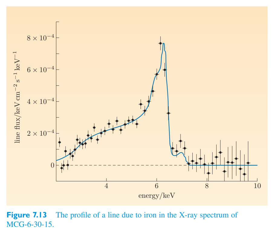
It is believed that quasars were common in all parts of the Universe when it was about a quarter of its present age. Each quasar, it is assumed, was powered by a supermassive black hole swallowing matter from its vicinity via an accretion disc. The black hole might have formed along with the galaxy or as the result of mergers between sub-galactic units. The prodigious amount of energy needed to account for the observed luminosity of a typical quasar is supposed to come from the release of gravitational potential energy by matter falling into the supermasive black hole. The gravitational potential energy would initially be converted to kinetic energy of the in-falling matter itself, but as the matter encountered and passed through the accretion disc, much of its kinetic energy would be converted to radiation. It is estimated that an in-fall rate of a few solar masses per year is enough to account for the luminosity of a typical quasar.人们相信类星体在宇宙的各个部分都很常见,当时它的年龄约为现在的四分之一。据推测,每个类星体都由一个超大质量黑洞提供动力,该黑洞通过吸积盘吞噬其附近的物质。黑洞可能是与星系一起形成的,或者是亚星系单元之间合并的结果。解释典型类星体的观测到的光度所需的巨大能量应该来自落入超大质量黑洞的物质释放的引力势能。引力势能最初会转化为下落物质本身的动能,但当物质遇到并穿过吸积盘时,其大部分动能将转化为辐射。据估计,每年几个太阳质量的下降率足以解释典型类星体的光度。
As the Universe aged, the galactic centre black holes responsible for quasar activity would have grown in mass while simultaneously clearing the space around them of consumable matter. In this way most quasars would have eventually exhausted their own fuel supply and ceased their activity. Most of those that we now observe are so distant that (due to the finite speed of light) we see them as they were long ago when still active. As for the smaller population of less remote quasars, it is assumed that either they have managed to remain active throughout cosmic history or they have been reactivated by a new supply of fuel, possibly as a result of a collision between galaxies. If this view is correct, quasar activity should be thought of as a phase through which galaxies pass rather than a characteristic of particular types of galaxy.随着宇宙的老化,负责类星体活动的银河中心黑洞的质量会增加,同时清除它们周围空间的消耗性物质。这样,大多数类星体最终会耗尽自身的燃料供应并停止活动。我们现在观察到的大多数星体都非常遥远,以至于(由于光速有限)我们看到的它们就像很久以前仍然活跃的样子。至于数量较少、距离较远的类星体,人们认为它们要么在整个宇宙历史中设法保持活跃,要么通过新的燃料供应重新激活,这可能是星系之间碰撞的结果。如果这种观点是正确的,那么类星体活动应该被认为是星系经过的一个阶段,而不是特定类型星系的特征。
The ‘youthful phase’ account of quasar activity is appealing as a story, but the scientific case for it recognizes two particularly important facts. First, galactic-scale collisions and mergers were common in the youthful Universe, making in-falling matter relatively abundant and thereby providing fuel for the quasar activity. Second, note the surprisingly high efficiency with which the accretion of matter converts gravitational potential energy to radiation. One way of defining the efficiency of an energy releasing process is as the ratio of the rate of energy release to the rate of fuel consumption expressed as the mass of fuel consumed per unit time multiplied by \(c^2\). (This definition of fuel consumption ensures that the efficiency will be the dimensionless ratio of two quantities with the same units, as it should be.) If we use L to denote the rate of radiative energy release (i.e. the luminosity), and \(c^2\) d m/d t for the rate of fuel consumption, the efficiency is类星体活动的“年轻阶段”描述作为一个故事很有吸引力,但它的科学案例认识到两个特别重要的事实。首先,银河系规模的碰撞和合并在年轻的宇宙中很常见,使得坠落物质相对丰富,从而为类星体活动提供燃料。其次,请注意物质的吸积将引力势能转化为辐射的效率惊人地高。定义能量释放过程的效率的一种方法是能量释放率与燃料消耗率的比率,表示为每单位时间消耗的燃料质量乘以\(c^2\)。(燃料消耗的这个定义确保效率将是具有相同单位的两个量的无量纲比,这应该是。)如果我们用 L 表示辐射能释放率(即光度),并用 \(c^2\) d m/d t 表示燃料消耗率,则效率为
In these terms, the most efficient energy releasing process is matter–antimatter annihilation, which has an efficiency of 1, or 100% if you prefer. The efficiency of gravitational energy release by accretion onto a black hole depends on the black hole’s rate of rotation; it varies from 5.7% for a non-rotating Schwarzschild black hole to 32% for a rapidly rotating Kerr black hole. This should be compared with an efficiency of only 0.7% for the nuclear fusion of hydrogen that is largely responsible for starlight. The overall situation as seen by astronomers in 2009 was described in an address by Royal Astronomical Society President, Andrew Fabian:从这些角度来看,最有效的能量释放过程是物质-反物质湮灭,其效率为 1,如果您愿意,也可以为 100%。黑洞吸积释放引力能的效率取决于黑洞的自转速率;它的变化范围从非旋转史瓦西黑洞的 5.7% 到快速旋转克尔黑洞的 32%。相比之下,氢核聚变的效率仅为 0.7%,而氢核聚变是星光的主要来源。英国皇家天文学会主席安德鲁·法比安 (Andrew Fabian) 在一次讲话中描述了 2009 年天文学家所看到的总体情况:
The visible sky is dominated by objects powered by nuclear fusion such as stars and galaxies. Shifting to shorter wavelengths in the X-ray band reveals an extragalactic sky powered by gravity: gravitational energy released by matter falling into black holes.... When accretion rates are high, considerable amounts of gravitational energy are released as radiation, and in some circumstances as powerful jets.可见的天空主要是由核聚变驱动的物体,例如恒星和星系。转向X射线波段的较短波长,揭示了由引力驱动的河外天空:落入黑洞的物质释放的引力能……当吸积率很高时,大量的引力能以辐射的形式释放,在某些情况下以强大的喷流的形式释放。
In summary, we have the following.总而言之,我们有以下几点。
Evidence from black holes来自黑洞的证据
There is good evidence for the existence of both stellar mass black holes and supermassive black holes. This includes indirect evidence of black hole rotation and the presence of an event horizon from analysis of a distorted iron line in the X-ray spectrum. This astronomical evidence gives further support to general relativity but does not provide a precise test.有充分的证据证明恒星质量黑洞和超大质量黑洞的存在。这包括黑洞旋转的间接证据以及通过对 X 射线光谱中扭曲铁线的分析得出的事件视界的存在。这些天文学证据进一步支持了广义相对论,但没有提供精确的测试。
Gravitational energy release through accretion onto black holes provides a plausible mechanism to account for the luminosity of quasars. The extragalactic X-ray sky is dominated by gravitationally powered sources.通过吸积到黑洞上释放的引力能提供了一种解释类星体光度的合理机制。河外 X 射线天空主要由引力驱动的源主导。
7.3.2 Gravitational lensing7.3.2 引力透镜
As described earlier, Einstein’s prediction of the gravitational deflection of light was first verified using data gathered in the total solar eclipse of 1919. The same physical process underlies the more recent discovery of gravitational lensing, the process in which a massive body (such as a galaxy or a cluster of galaxies), located between an observer and a distant source of electromagnetic radiation, causes the observer to see distorted or multiple images of the source.如前所述,爱因斯坦对光的引力偏转的预测首先通过 1919 年日全食收集的数据得到验证。同样的物理过程是最近发现的引力透镜的基础,在该过程中,位于观察者和遥远的电磁辐射源之间的大质量物体(例如星系或星系团)使观察者看到源的扭曲或多个图像。
In 1979, Dennis Walsh (1933–2005) and his colleagues pointed out that two narrowly separated quasars, Q0957+561 A and B (which we shall simply refer to as A and B), have identical optical and radio spectra. They are evidently at the same distance since their spectra are redshifted by the same amount. The most likely interpretation seemed to be that A and B are actually two images of a single quasar and that the light from that quasar is reaching the Earth by two different paths due to gravitational lensing (Figure 7.14).1979年,丹尼斯·沃尔什(Dennis Walsh,1933-2005)和他的同事指出,两个距离很近的类星体Q0957+561 A和B(我们简称为A和B)具有相同的光学和射电光谱。它们显然处于相同的距离,因为它们的光谱红移了相同的量。最可能的解释似乎是,A 和 B 实际上是单个类星体的两个图像,并且由于引力透镜作用,来自该类星体的光通过两条不同的路径到达地球(图 7.14)。
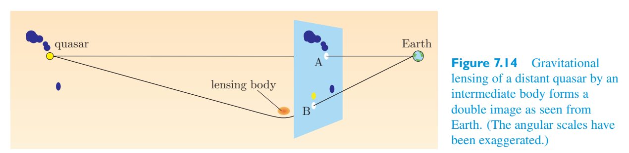
The body responsible for the lensing was shown to be a galaxy, faint but detectable, located between the quasar and the Earth. This was the first example of a gravitational lens. It should be understood that a gravitational lens is not a true ‘lens’ in the optical sense of that term. Figure 7.15 shows the action of a converging optical lens on parallel rays, representing light from a source at an effectively infinite distance. In the case of an optical lens, the deflection of light increases with increasing distance from the central axis. Contrast that with the behaviour of parallel light rays passing a massive body, as shown in Figure 7.16.造成透镜效应的物体被证明是一个星系,虽然微弱但可探测到,位于类星体和地球之间。这是引力透镜的第一个例子。应该理解的是,引力透镜并不是光学意义上的真正的“透镜”。图 7.15 显示了会聚光学透镜对平行光线的作用,代表来自实际上无限远距离的光源的光。在光学透镜的情况下,光的偏转随着距中心轴的距离的增加而增加。将其与平行光线穿过大质量物体的行为进行对比,如图 7.16 所示。
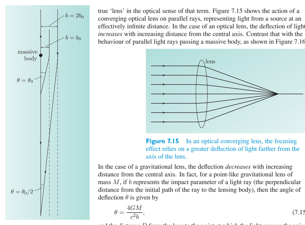
In the case of a gravitational lens, the deflection decreases with increasing distance from the central axis. In fact, for a point-like gravitational lens of mass M, if b represents the impact parameter of a light ray (the perpendicular distance from the initial path of the ray to the lensing body), then the angle of在引力透镜的情况下,偏转随着距中心轴距离的增加而减小。事实上,对于质量为M的点状引力透镜,如果b代表光线的撞击参数(光线初始路径到透镜体的垂直距离),那么
and the distance D from the lens to the point at which the light crosses the axis is given by从透镜到光穿过轴的点的距离 D 由下式给出
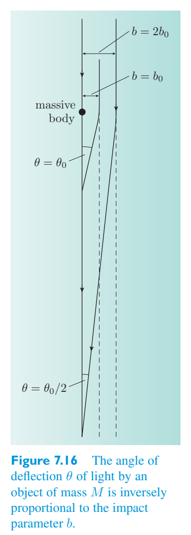
The theory of gravitational lenses is very different from that of ordinary lenses. Real images of extended objects are never seen. Any intervening body of sufficient mass (such as a black hole) can produce gravitational lensing. If a point source, intervening body and observer all happened to be exactly in line, then the source would appear as a ring. Such circumstances do occur, but it is much more common to see a series of arcs or blobs. Figure 7.17 shows a picture taken by the Hubble space telescope of an object known as the ‘Einstein cross’ that includes four images of a distant quasar and a central image of the lensing body. An additional effect is that the light from the different images may arrive at different times (up to weeks apart) due to taking different optical paths and experiencing different spacetime curvature (this is another manifestation of the Shapiro time delay effect).引力透镜的理论与普通透镜有很大不同。扩展物体的真实图像从未见过。任何具有足够质量的介入体(例如黑洞)都可以产生引力透镜。如果点源、介入体和观察者恰好恰好在一条线上,那么源将显示为一个环。这种情况确实会发生,但更常见的是看到一系列弧线或斑点。图 7.17 显示了哈勃太空望远镜拍摄的一个被称为“爱因斯坦十字”的物体的照片,其中包括遥远类星体的四张图像和透镜体的中心图像。另一个效果是,由于采用不同的光路并经历不同的时空曲率,来自不同图像的光可能会在不同的时间到达(最多相隔数周)(这是夏皮罗时间延迟效应的另一种表现)。
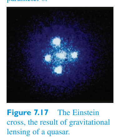
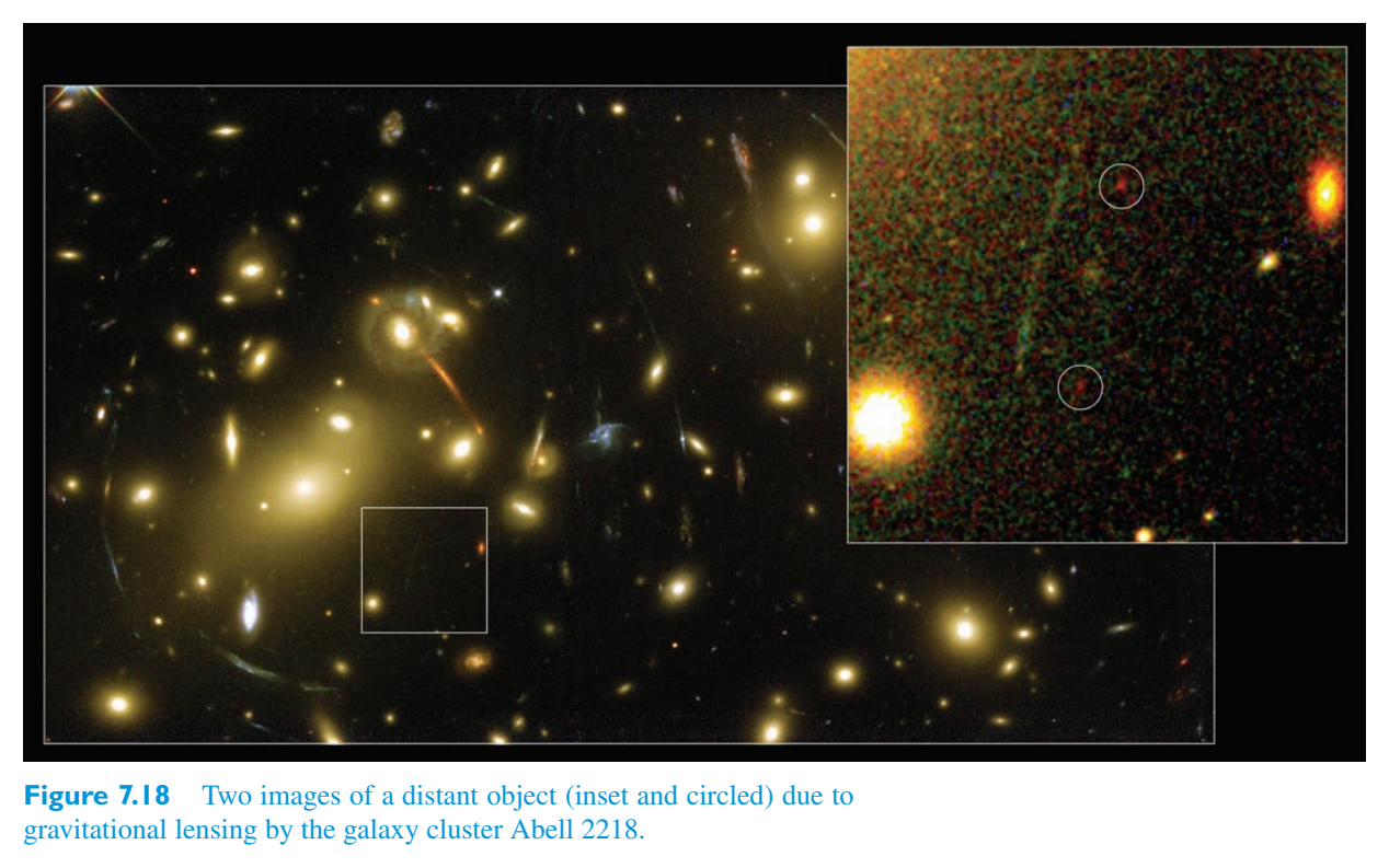
Gravitational lensing affects all electromagnetic radiation and has also been observed at radio and X-ray wavelengths. It provides support for general relativity but is not really a stringent test of the theory. Rather it is a useful observational tool with many applications. For example, a gravitational lens may concentrate the light of a faint object to bring it above the threshold of what is detectable. In this context, the object known as Abell 2218, a rich cluster of galaxies located about 2 billion light-years away, enables a far more distant object to be detected, as shown in Figure 7.18. The Abell 2218 cluster has produced two images of the distant object (circled in the inset) and amplified the brightness of each by a factor of about 30.引力透镜影响所有电磁辐射,并且在无线电和 X 射线波长下也被观察到。它为广义相对论提供了支持,但实际上并不是对该理论的严格检验。相反,它是一种有用的观察工具,具有许多应用。例如,引力透镜可以集中微弱物体的光,使其高于可检测的阈值。在这种情况下,被称为 Abell 2218 的天体(一个距离我们约 20 亿光年的丰富星系团)使得能够探测到更遥远的天体,如图 7.18 所示。 Abell 2218 星团生成了两个遥远物体的图像(插图中圈出的图像),并将每个图像的亮度放大了约 30 倍。
Exercise 7.6 A gravitational lens does not function in the same way as a练习 7.6 引力透镜的作用与引力透镜不同
converging optical lens. Explain in qualitative terms how, notwithstanding this, the brightness of a very distant object can be amplified by a factor of 30 due to gravitational lensing.会聚光学透镜。尽管如此,还是用定性术语解释一下,如何通过引力透镜将非常远的物体的亮度放大 30 倍。
The term gravitational lensing is usually applied to situations in which the lensing body is very massive, typically a galaxy or a cluster of galaxies. However, the process is a general one and there is no reason, in principle, why the lensing body should not be much smaller. In fact, gravitational lensing by bodies of stellar mass or less has been observed since the early 1990s and is generally referred to as gravitational microlensing. When dealing with lensing bodies of such low mass it is not practical to detect image distortion, so image brightening is used instead. The technique is straightforward: bright stars in a nearby galaxy are carefully and continuously monitored using equipment capable of recording fluctuations in brightness. If a dense dark body passes across the line of sight from the observing site to any one of the monitored stars, then the brightness of that star will change and its variation with time can be recorded as a light curve. There are many reasons why the brightness of a stellar body might change, but microlensing will produce a characteristic contribution that can be distinguished from other signals and used to model the properties of the lensing body. In this way it is possible to search for isolated stellar mass black hole candidates and to put limits on the abundance of stellar mass black holes in the outer parts of the Milky Way.术语“引力透镜”通常适用于透镜体质量非常大的情况,通常是一个星系或星系团。不过,这一过程是普遍的;原则上没有理由认为透镜体不能小得多。事实上,自 20 世纪 90 年代初以来,人们就观察到了恒星质量或更小的天体的引力透镜,通常被称为引力微透镜效应。当处理如此低质量的透镜体时,检测图像失真是不切实际的,因此使用图像增亮来代替。这项技术很简单:使用能够记录亮度波动的设备仔细、连续地监测附近星系中的明亮恒星。如果一个致密的暗体从观测地点穿过视线到达任何一颗被监测的恒星,那么该恒星的亮度就会发生变化,并且它随时间的变化可以被记录为光变曲线。恒星体亮度发生变化的原因有很多,但微透镜会产生一种特征贡献,可以与其他信号区分开来,并用于模拟透镜体的特性。通过这种方式,可以寻找孤立的恒星质量黑洞候选者,并限制银河系外部恒星质量黑洞的丰度。
Evidence from gravitational lensing来自引力透镜的证据
There are many examples of gravitational lenses. These give additional support to general relativity.引力透镜的例子有很多。这些为广义相对论提供了额外的支持。
7.4 Gravitational waves7.4 引力波
In 1993 the Nobel Prize for Physics was awarded to Joseph Taylor (1941–) and his former graduate student Russell Hulse (1950–) for their discovery (in 1974) and subsequent study of a very unusual binary star system that has become a test-bed for general relativity. The Hulse–Taylor system is believed to consist of two neutron stars, one of which is emitting regular pulses of radiation at radio wavelengths and is therefore classified as a pulsar and designated PSR B1913+16. Pulsars were first detected in the 1960s by Jocelyn Bell Burnell (1943–) and it was soon proposed that they were actually rapidly rotating neutron stars with a strong magnetic field. Many are now known but PSR B1913+16 was the first binary pulsar — a pulsar confirmed as part of a close binary system. In the Hulse–Taylor system, both of the compact stars has a mass of about 1.4 M), and the pair orbit each other with a period of just 7.75 hours. The star that is a pulsar is thought to turn on its axis 17 times per second, accounting for the observed pulse separation of 59 milliseconds.1993 年,诺贝尔物理学奖授予约瑟夫·泰勒(Joseph Taylor,1941 年至今)和他以前的研究生拉塞尔·赫尔斯(Russell Hulse,1950 年至今),以表彰他们发现(1974 年)并随后研究了一个非常不寻常的双星系统,该系统已成为广义相对论的试验台。赫尔斯-泰勒系统被认为由两颗中子星组成,其中一颗发射无线电波长的规则辐射脉冲,因此被归类为脉冲星,并指定为 PSR B1913+16。脉冲星在 20 世纪 60 年代首次被乔斯林·贝尔·伯内尔 (Jocelyn Bell Burnell,1943-) 发现,很快人们就提出它们实际上是具有强磁场的快速旋转的中子星。现在许多脉冲星已为人所知,但 PSR B1913+16 是第一个双星脉冲星——一颗脉冲星被确认为封闭双星系统的一部分。在赫尔斯-泰勒系统中,两颗致密星的质量约为 1.4 M),且这两对恒星绕对方运行的周期仅为 7.75 小时。据认为,这颗脉冲星恒星每秒绕轴转动 17 次,因此观测到的脉冲间隔为 59 毫秒。
According to general relativity, a system of this kind should mainly lose energy through the emission of gravitational waves, a form of radiation involving propagating distortions of spacetime that was proposed by Einstein in 1916. As a result of gravitational wave emission, the orbital period of PSR B1913+16 should be decreasing in a predictable way. This prediction has now been tested over more than three decades and has been found to accurately agree with observations to within 0.2% (see Figure 7.19). It is an impressive confirmation of general relativity and also an indirect confirmation of the existence of gravitational waves, which have still not been directly detected here on Earth. (Note that gravitational radiation has nothing to do with electromagnetic waves and is not part of the electromagnetic spectrum. The Hulse–Taylor system is observed using electromagnetic (radio) waves, even though its orbital decay is mainly attributed to the emission of gravitational waves.)根据广义相对论,这种系统主要通过引力波的发射来损失能量,引力波是爱因斯坦于 1916 年提出的一种涉及时空传播扭曲的辐射形式。由于引力波发射,PSR B1913+16 的轨道周期应该以可预测的方式减少。这一预测现已经过三十多年的检验,结果与观测值的准确度一致,误差在 0.2% 以内(见图 7.19)。这是对广义相对论的令人印象深刻的证实,也是对引力波存在的间接证实,而引力波在地球上尚未被直接探测到。(请注意,引力辐射与电磁波无关,也不属于电磁波谱的一部分。赫尔斯-泰勒系统是使用电磁(无线电)波观测的,尽管其轨道衰变主要归因于引力波的发射。)
This section is devoted to gravitational waves. It starts by introducing gravitational waves as solutions of the Einstein field equations and then goes on to examine the methods that may be used to detect them and some of the likely sources of such waves.本节专门讨论引力波。首先介绍引力波作为爱因斯坦场方程的解,然后继续研究可用于检测它们的方法以及此类波的一些可能来源。
7.4.1 Gravitational waves and the Einstein7.4.1 引力波和爱因斯坦
field equations场方程
In regions of spacetime where the gravitational field is weak, the curvature will be small and the metric tensor can be written as h \(\mu\)\(\nu\) is small, we can make the simplification that we only retain terms linear in h \(\mu\)\(\nu\). This means that in the case of weak fields, the Einstein field equations在引力场较弱的时空区域,曲率会很小,度规张量可以写为 h \(\mu\)\(\nu\) 很小,我们可以简化为只保留 h \(\mu\)\(\nu\) 中的线性项。这意味着在弱场的情况下,爱因斯坦场方程
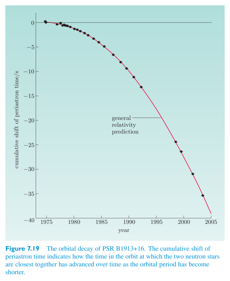
can be represented by the linearized field equation可以用线性化场方程表示
and the box symbol represents a combination of derivatives that is frequently c: encountered when dealing with waves that travel with speed方框符号表示在处理高速传播的波时经常遇到的导数组合
It should be pointed out that the indices in Equation 7.17 are (by definition) raised and lowered using the Minkowski metric tensor [\(\eta\) \(\mu\)\(\nu\)], so Equation 7.17 genuinely is linear in h \(\mu\)\(\nu\). This linear equation has wave-like solutions, but that is far from obvious, partly due to the effect of gauge symmetry.应该指出的是,方程 7.17 中的指数(根据定义)是使用闵可夫斯基度规张量 [\(\eta\) \(\mu\)\(\nu\)] 升高和降低的,因此方程 7.17 在 h \(\mu\)\(\nu\) 中确实是线性的。这个线性方程具有类似波的解,但这远非显而易见,部分原因是规范对称性的影响。
You may recall that when we discussed the Maxwell equations in Chapter 2, we said that the theory of electromagnetism contained an important symmetry called gauge symmetry. A related symmetry arises in general relativity. It is present in Equation 7.17 and prevents us from solving the equation in any simple way. In order to find an explicit solution, it is necessary to impose a condition that removes the effect of this symmetry. This extra condition is said to ‘fix’ the gauge. There are many ways of fixing the gauge; a common one is to define the quantity你可能还记得,当我们在第二章讨论麦克斯韦方程时,我们说过电磁学理论包含一个重要的对称性,称为规范对称性。广义相对论中出现了相关的对称性。它出现在方程 7.17 中,并阻止我们以任何简单的方式求解方程。为了找到显式解,有必要施加一个条件来消除这种对称性的影响。据说这个额外的条件可以“修复”仪表。固定仪表的方法有很多种;常见的一个是定义数量
and then impose the condition然后施加条件
This leads to the greatly simplified linearized field equation这导致线性化场方程大大简化
This kind of differential equation is well known in the study of waves. It is described as an inhomogeneous wave equation with a source term (− 2 \(\kappa\) \(T_{\mu\nu}\)). It implies that gravitational waves can be generated by a source that changes in an appropriate way. (The Hulse–Taylor system is such a source, but a body that changes in a spherically symmetric way is not.) In a region where there are no sources, the spacetime disturbances are described by the homogeneous wave equation! h \(\mu\)\(\nu\) = 0, which is satisfied by waves that travel with speed c.这种微分方程在波浪研究中是众所周知的。它被描述为具有源项 (− 2 \(\kappa\) \(T_{\mu\nu}\)) 的非齐次波动方程。这意味着引力波可以由以适当方式变化的源产生。(赫尔斯-泰勒系统就是这样的源,但以球对称方式变化的物体则不是。)在没有源的区域中,时空扰动由齐次波动方程描述! h \(\mu\)\(\nu\) = 0,以速度 c 传播的波满足该条件。
It might appear from what has been said that gauge invariance is simply an unfortunate inconvenience. However, this is far from being true. In both electromagnetism and general relativity, the gauge symmetry is a very deep and fundamental property of the theory.从上述内容看来,规范不变性只是一种不幸的不便。然而,事实并非如此。在电磁学和广义相对论中,规范对称性是理论的一个非常深刻和基本的属性。
- ● Which theorem introduced earlier ensures that a star that collapses in a前面介绍的哪个定理确保了恒星在
spherically symmetric way cannot be a source of gravitational waves? Explain the reason for your answer.球对称方式不能成为引力波源吗?解释你的答案的原因。
❍ Birkhoff’s theorem. This ensures that the solution exterior to a spherically symmetric body (even one that is collapsing) must be described by the Schwarzschild metric. Since that metric is stationary, it cannot describe a gravitational wave, which will necessarily be described by a non-stationary metric.伯克霍夫定理。这确保了球对称体(即使是正在塌陷的球对称体)外部的解必须由史瓦西度规来描述。由于该度规是平稳的,因此它不能描述引力波,而引力波必须用非平稳度规来描述。
7.4.2 Methods of detecting gravitational waves7.4.2 探测引力波的方法
We have already seen that the indirect observation of gravitational waves has almost certainly been achieved through the study of the Hulse–Taylor binary pulsar. The problem, then, is the direct detection of gravitational waves.我们已经看到,通过对赫尔斯-泰勒双脉冲星的研究,几乎可以肯定已经实现了对引力波的间接观测。那么,问题就在于引力波的直接探测。
The existence of electromagnetic waves (predicted by Maxwell’s equations) was dramatically confirmed by Heinrich Hertz (1857–1894) when he generated such waves in the laboratory using non-steady currents. One could imagine trying to generate gravitational waves in the laboratory by rapidly moving a massive object. Unfortunately, it turns out that if one rotates a bar of steel weighing several tons to the point where it is about to split apart under centrifugal forces, one radiates only about 10 − 30 W. For this reason, current experiments attempt to detect gravitational waves generated by large-scale astronomical events, such as supernovae or mergers of decaying binary systems.当海因里希·赫兹(Heinrich Hertz,1857-1894)在实验室中使用非稳态电流产生电磁波时,他戏剧性地证实了电磁波的存在(由麦克斯韦方程组预测)。人们可以想象在实验室中通过快速移动一个巨大的物体来产生引力波。不幸的是,事实证明,如果将一根重达数吨的钢棒旋转到在离心力作用下即将分裂的程度,其辐射强度仅为约 10 - 30 W。因此,当前的实验试图探测大规模天文事件(例如超新星或衰变双星系统的合并)产生的引力波。
Attempts have been made to detect gravitational waves since the 1960s. All are based on attempting to detect the relative movement of massive bodies caused by the rippling of spacetime as the wave passes through the apparatus. The massive bodies can be either the parts of an elastic body, in which case it is anticipated that the wave would create a resonance akin to the ringing of a bell, or ‘free particles’, where the relative movement of the individual particles can be detected.自 20 世纪 60 年代以来,人们一直在尝试探测引力波。所有这些都是基于试图检测当波穿过设备时由时空波纹引起的大质量物体的相对运动。大质量物体可以是弹性体的一部分,在这种情况下,预计波会产生类似于钟声的共振,也可以是“自由粒子”,其中可以检测到单个粒子的相对运动。
The earliest experiments were of the elastic body type and made use of what is known as a resonant bar detector (sometimes called a Weber bar) — a large metal bar equipped with sensors to measure tiny movements of the ends (Figure 7.20). The idea was that the effect of a gravitational wave would be amplified by the resonant frequency of the bar and hence produce a measurable change in the distance between the ends. Although modern versions of this device are in operation, they are not sensitive enough to measure anything other than an extremely powerful and therefore very rare gravitational wave.最早的实验是弹性体类型,并使用所谓的共振棒探测器(有时称为韦伯棒)——一种配备传感器的大型金属棒,用于测量末端的微小运动(图 7.20)。这个想法是,引力波的影响会被棒的共振频率放大,从而在两端之间的距离产生可测量的变化。尽管该设备的现代版本正在运行,但它们的灵敏度不够高,无法测量除了极其强大且非常罕见的引力波之外的任何东西。
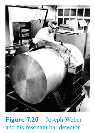
Most modern detectors are of the ‘free particle’ type since that has a greater potential for detecting the less powerful signals that are almost certainly more common. There are currently several gravitational wave detectors of this type in operation, but the most sensitive is LIGO, the Laser Interferometer Gravitational-Wave Observatory.大多数现代探测器都是“自由粒子”类型,因为它更有潜力检测到几乎肯定更常见的较弱信号。目前有多个此类引力波探测器正在运行,但最灵敏的是 LIGO(激光干涉仪引力波天文台)。
LIGO uses laser interferometers to monitor changes in the separation of suspended mirrors. As shown in Figure 7.21 overleaf, the interferometer consists of two ‘light storage arms’ at right angles forming an ‘L’ shape. Each arm has a mirror at either end so that light can repeatedly bounce back and forth. A laser supplies the light, which enters the arms via a beam splitter located at the corner of the L. In simple terms, if the arms are of constant length, the system can be arranged so that interference between the light beams returning to the beam splitter will direct all of the light back towards the laser. However, if either arm changes its length, the interference pattern will change and some light will reach the photodetector, where it can be recorded. When in operation, LIGO seeks changes in the lengths of the arms as revealed by alterations in the signal from the photodetector. The key challenge is to distinguish the very tiny signal from the unavoidable noise.LIGO 使用激光干涉仪来监测悬浮镜分离的变化。如图 7.21 背面所示,干涉仪由两个呈直角形成“L”形的“光存储臂”组成。每条手臂的两端都有一面镜子,这样光线就可以反复来回反射。激光提供光线,光线通过位于 L 角的分束器进入手臂。简单来说,如果臂的长度恒定,则系统可以布置成使得返回分束器的光束之间的干涉将引导所有光返回激光器。然而,如果任一臂改变其长度,干涉图案就会改变,一些光将到达光电探测器,并在那里被记录下来。在运行时,LIGO 会通过光电探测器信号的变化来寻找臂长度的变化。关键的挑战是区分非常微小的信号和不可避免的噪声。
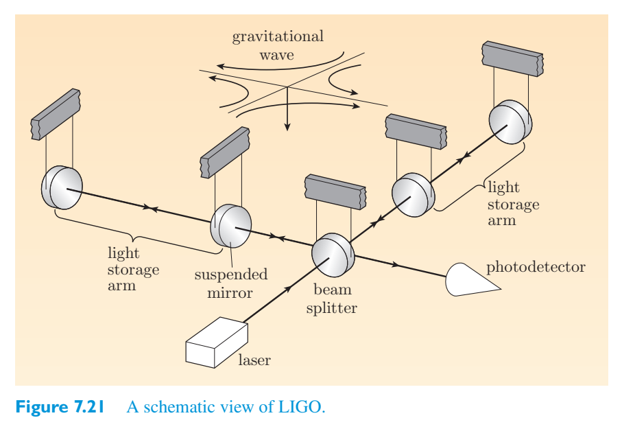
beams travel in highly a likely gravitational − 18 m, which is less than relative change in distance光束在很可能的引力范围内传播 - 18 m,小于距离的相对变化
interferometers — two at the state of Washington, LIGO has should enable a Since gravitational waves separation corresponds to Triangulation should of the source.干涉仪——位于华盛顿州的两个干涉仪,LIGO 应该能够实现引力波分离,因为引力波分离对应于源的三角测量。
any gravitational任何引力
LIGO, which will expected to be operational including LISA a joint project between interferometer consisting triangle with sides of about 5 million kilometres, as shown in Figure 7.22. LISA will be sensitive to gravitational waves at a lower frequency than LIGO, so the two experiments should complement each other. It is currently expected that the spacecraft will be launched in 2019 or 2020 and the project will last about 5 to 8 years.LIGO 预计将投入运行,包括 LISA 干涉仪之间的联合项目,该项目由边长约 500 万公里的三角形组成,如图 7.22 所示。 LISA 对频率低于 LIGO 的引力波敏感,因此这两个实验应该相辅相成。目前预计该航天器将于2019年或2020年发射,项目将持续约5至8年。
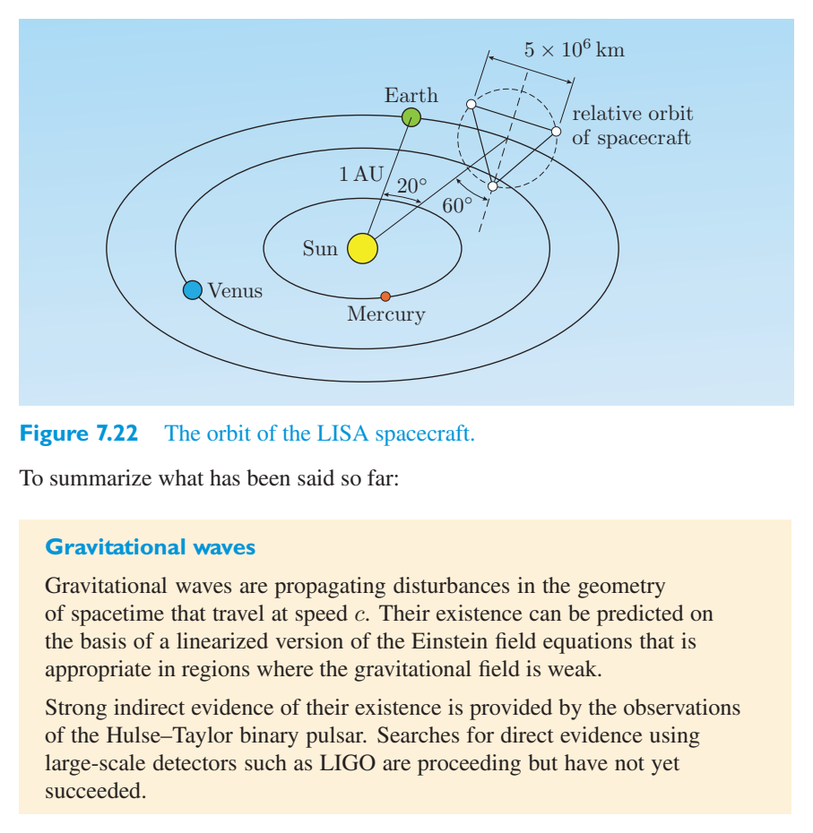
Gravitational waves引力波
Gravitational waves are propagating disturbances in the geometry of spacetime that travel at speed c. Their existence can be predicted on the basis of a linearized version of the Einstein field equations that is appropriate in regions where the gravitational field is weak.引力波是以速度 c 传播的时空几何形状的扰动。它们的存在可以根据爱因斯坦场方程的线性化版本来预测,该方程适用于引力场较弱的区域。
Strong indirect evidence of their existence is provided by the observations of the Hulse–Taylor binary pulsar. Searches for direct evidence using large-scale detectors such as LIGO are proceeding but have not yet succeeded.对赫尔斯-泰勒双脉冲星的观测提供了它们存在的强有力的间接证据。使用 LIGO 等大型探测器寻找直接证据的工作正在进行中,但尚未成功。
7.4.3 Likely sources of gravitational waves7.4.3 引力波的可能来源
Gravitational waves and supernovae One of the expected sources of gravitational waves is supernova explosions in neighbouring galaxies. Indeed, the target sensitivities of some existing gravitational detectors have been set with this in mind. Gravitational waves from a supernova explosion in a galaxy in the rich Virgo cluster of galaxies (centred about 60 million light years away) would cause a change of about 1 part in \(10^{21}\) in lengths on Earth, and this is the target sensitivity of LIGO. As mentioned earlier, if the collapse of the star in a supernova is spherically symmetric, then there will be no gravitational radiation. However, it is thought that supernovae, particularly in binary systems, are asymmetric.引力波和超新星引力波的预期来源之一是邻近星系中的超新星爆炸。事实上,一些现有引力探测器的目标灵敏度就是考虑到这一点而设定的。丰富的室女座星系团(中心距离约 6000 万光年)的超新星爆炸产生的引力波会导致地球长度约 \(10^{21}\) 的 1 分之一变化,这就是 LIGO 的目标灵敏度。正如前面提到的,如果超新星中恒星的塌缩是球对称的,那么就不会有引力辐射。然而,人们认为超新星,特别是双星系统中的超新星,是不对称的。
Gravitational waves and black holes A possible source of gravitational waves would involve two black holes in orbit about each other. Such an orbiting pair would steadily emit gravitational radiation, eventually culminating in a huge burst as they fused into a single black hole. While the final black hole would, by virtue of the ‘no hair theorem’, be indistinguishable from any other black hole of the same mass and angular momentum, the outgoing ripples in spacetime would have encoded in them an account of the process in which they were emitted. This would be a very distinctive signal for the existence of black holes.引力波和黑洞引力波的一个可能来源是两个围绕彼此轨道运行的黑洞。这样的轨道对会稳定地发射引力辐射,最终在它们融合成一个黑洞时产生巨大的爆发。虽然根据“无毛定理”,最终的黑洞与具有相同质量和角动量的任何其他黑洞无法区分,但时空中传出的涟漪会在其中编码它们发射过程的描述。这将是黑洞存在的一个非常独特的信号。
Gravitational waves and cosmology Gravitational waves of a wide spectrum of frequencies are expected from the ‘quantum fluctuations’ in the metric of spacetime that occurred during the Big Bang. The observation of gravitational waves should throw light on a central problem of modern cosmology: the origin of the density fluctuations that eventually led to a lumpy Universe (i.e. one containing galaxies) rather than a perfectly uniform one. The large-scale structure of the Universe is central to the next chapter, which is devoted to relativistic cosmology.引力波和宇宙学大爆炸期间发生的时空度规的“量子涨落”预计会产生宽频谱的引力波。对引力波的观测应该能够揭示现代宇宙学的一个核心问题:密度涨落的起源,最终导致了一个块状的宇宙(即包含星系的宇宙),而不是一个完全均匀的宇宙。宇宙的大尺度结构是下一章的核心,这一章专门讨论相对论宇宙学。
Summary of Chapter 7第 7 章总结
1. The four classic tests of general relativity are as follows.1. 广义相对论的四个经典检验如下。
(a) The precession of the perihelion of Mercury The observations, which have an uncertainty of about 1%, are consistent with the predictions of general relativity.(a) 水星近日点进动观测结果与广义相对论的预测一致,不确定度约为1%。
(b) Deflection of light by the Sun The observations, which have an experimental uncertainty of about 10% for optical wavelengths, are in agreement with the predictions of general relativity. The agreement is better than 0.04% for VLBI radio telescope observations.(b) 太阳对光的偏转这些观测结果与广义相对论的预测一致,其光学波长的实验不确定度约为 10%。 VLBI 射电望远镜观测结果的一致性优于 0.04%。
(c) Gravitational redshift Gravitational redshift has been verified to better than 1% in variants of the Pound–Rebka experiment. Gravity Probe A verified the time dilation due to general relativity to 70 parts per million. The continued functioning of the GPS confirms general relativistic time dilation to about 1% on a daily basis.(c) 引力红移在 Pound-Rebka 实验的变体中,引力红移已被证实优于 1%。引力探测器 A 验证了广义相对论引起的时间膨胀达到百万分之 70。 GPS 的持续运行证实了广义相对论时间每天膨胀约 1%。
(d) Time delay of electromagnetic radiation passing the Sun The Cassini probe confirmed the effect to about 20 parts per million.(d) 电磁辐射穿过太阳的时间延迟卡西尼号探测器证实了这种效应约为百万分之二十。
2. Satellite-based tests aim to detect two effects:2. 基于卫星的测试旨在检测两种效果:
- • geodesic gyroscope precession• 测地陀螺进动
- • frame dragging (Lense–Thirring effect).• 帧拖动(Lense–Thirring 效果)。
Two satellite-based tests are:两项基于卫星的测试是:
(a) The LAGEOS satellite results, which have been claimed to confirm frame dragging to 10%, but this is disputed.(a) LAGEOS 卫星结果,据称证实帧拖拽达到 10%,但这一点存在争议。
(b) Gravity Probe B results, which confirm geodesic gyroscope precession to 1.5%. The expected frame dragging is below the noise level, though there is still some hope that further analysis might improve the situation.(b) 引力探测器 B 结果,确认测地陀螺仪进动为 1.5%。预期的帧拖拽低于噪声水平,但仍有希望进一步分析可以改善这种情况。
3. There is good evidence for the existence of both stellar3. 有充分的证据证明这两颗恒星的存在
mass black holes and supermassive black holes. This includes indirect evidence of black hole rotation and the presence of an event horizon from analysis of a distorted iron line in the X-ray spectrum. This astronomical evidence gives further support to general relativity but does not provide a precise test.质量黑洞和超大质量黑洞。这包括黑洞旋转的间接证据以及通过对 X 射线光谱中扭曲铁线的分析得出的事件视界的存在。这些天文学证据进一步支持了广义相对论,但没有提供精确的测试。
4. Gravitational energy release through accretion onto black holes provides a4. 通过吸积到黑洞上释放的引力能提供了
plausible mechanism to account for the luminosity of quasars. The extragalactic X-ray sky is dominated by gravitationally powered sources.解释类星体光度的合理机制。河外 X 射线天空主要由引力驱动的源主导。
5. There are many examples of gravitational lenses. These give additional5. 引力透镜的例子有很多。这些给予额外的
support to general relativity.支持广义相对论。
6. Gravitational waves are propagating disturbances in the geometry of6. 引力波是在几何形状中传播的扰动
spacetime that travel at speed c. Their existence can be predicted on the basis of a linearized version of the Einstein field equations that is appropriate in regions where the gravitational field is weak.以一定速度传播的时空 C.它们的存在可以根据爱因斯坦场方程的线性化版本来预测,该方程适用于引力场较弱的区域。
(a) The orbital decay of the binary pulsar PSR B1913+16 has been observed for over 30 years and is consistent with the expected loss of energy due to the emission of gravitational waves as predicted by general relativity.(a) 双脉冲星 PSR B1913+16 的轨道衰变已被观测了 30 多年,与广义相对论预测的由于引力波发射而导致的能量损失一致。
(b) Although no gravitational waves have been directly detected to date (2009), it is expected that they are created by large-scale astronomical events, provided that they are not spherically symmetric.(b) 虽然迄今为止(2009年)尚未直接探测到引力波,但预计它们是由大规模天文事件产生的,只要它们不是球对称的。
(c) Currently, the most sensitive detector is LIGO, the Laser Interferometer Gravitational-Wave Observatory, which has been designed to be able to detect a supernova in the Virgo cluster of galaxies. Advanced LIGO should increase the sensitivity by a factor of 100 and is expected to be operational by 2014.(c) 目前,最灵敏的探测器是 LIGO,即激光干涉引力波天文台,其设计目的是能够探测室女座星系团中的超新星。高级 LIGO 的灵敏度应提高 100 倍,预计将于 2014 年投入运行。
Chapter 8 Relativistic cosmology第8章相对论宇宙学
Introduction介绍
Cosmology is the study of the Universe as a whole, including its origin, nature, evolution and eventual fate. It has ancient roots in philosophy and religion, but modern scientific cosmology dates from 1917 when Einstein first used general relativity to formulate a mathematical model of the Universe.宇宙学是对整个宇宙的研究,包括其起源、本质、演化和最终命运。它有着古老的哲学和宗教根源,但现代科学宇宙学可以追溯到 1917 年,当时爱因斯坦首次使用广义相对论来制定宇宙的数学模型。
Einstein was not an astronomer, so he sought astronomical advice before attempting to apply general relativity on the cosmic scale. Actually, little was known about the large-scale structure of the Universe at the time, so Einstein was led to formulate a static model, nether expanding nor contracting, that is now known to disagree with observational evidence. As a result, the details of Einstein’s original model are mainly of historical interest. Nonetheless, his basic approach, of formulating a mathematical model describing the large-scale features of the Universe, usually called a cosmological model, still provides the basis of modern relativistic cosmology.爱因斯坦不是天文学家,因此他在尝试将广义相对论应用于宇宙尺度之前寻求天文学建议。事实上,当时人们对宇宙的大尺度结构知之甚少,因此爱因斯坦被引导制定了一个既不膨胀也不收缩的静态模型,现在已知该模型与观测证据不符。因此,爱因斯坦原始模型的细节主要具有历史意义。尽管如此,他建立描述宇宙大尺度特征的数学模型(通常称为宇宙学模型)的基本方法仍然为现代相对论宇宙学提供了基础。
Cosmology is now a booming subject. Much of the subject’s recent success has been the result of developments in our understanding of the physics of elementary particles and rapid progress in observational astronomy. It is impossible to do justice to either of these topics in one short chapter. Fortunately, the cosmological aspects of both are covered more fully in this book’s companion volume, Observational cosmology by Stephen Serjeant. Consequently, the current chapter mainly provides an introduction to those aspects of cosmology that relate directly to general relativity and only includes a minimum of observational information.宇宙学现在是一个蓬勃发展的学科。该学科最近的成功很大程度上归功于我们对基本粒子物理学的理解的发展以及观测天文学的快速进步。在短短的一章中不可能公正地阐述这些主题中的任何一个。幸运的是,这本书的姊妹篇《观测宇宙学》(作者:Stephen Serjeant)更全面地介绍了两者的宇宙学方面。因此,本章主要介绍宇宙学中与广义相对论直接相关的方面,并且仅包含最少的观测信息。
The first section concerns the basic principles that underlie modern relativistic cosmology. These are approached from a mainly physical perspective and set the scene for a section devoted to the standard mathematical model of spacetime on the cosmological scale. That model takes the form of a specific metric known as the Robertson–Walker metric that, like the Schwarzschild metric, is usually presented as a four-dimensional spacetime line element. Having discussed spacetime on the cosmic scale, we next turn to the contents of that spacetime. As is conventional in cosmology, we treat the contents of spacetime as consisting essentially of matter and radiation, but when we come to write down an energy–momentum tensor for the Universe, we shall also include a contribution from the dark energy or cosmological constant that was mentioned at the end of Chapter 4. Accepting that Einstein’s notion of a static Universe was wrong, our main aim in the third section is to use the Einstein field equations to derive the Friedmann equations that describe the evolution of the Universe. The Friedmann equations achieve this by relating the large-scale geometric features of spacetime to the large-scale distribution of energy and momentum. The combination of Robertson–Walker spacetime with matter, radiation and dark energy that evolve in accordance with the Friedmann equations results in a class of cosmological models known as the Friedmann–Robertson–Walker models. The final section of this chapter considers the observational consequences of supposing that the Universe we inhabit is well described by a Friedmann–Robertson–Walker model, and thereby provides a link to the companion volume on observational cosmology.第一部分涉及现代相对论宇宙学的基本原理。这些主要从物理角度进行探讨,并为专门讨论宇宙尺度上的时空标准数学模型的部分奠定了基础。该模型采用称为罗伯逊-沃克度规的特定度规形式,与史瓦西度规一样,通常表示为四维时空线元素。讨论了宇宙尺度的时空之后,我们接下来讨论时空的内容。按照宇宙学的惯例,我们将时空的内容视为本质上由物质和辐射组成,但是当我们写下宇宙的能量-动量张量时,我们还应包括第四章末尾提到的暗能量或宇宙学常数的贡献。承认爱因斯坦的静态宇宙概念是错误的,我们在第三部分的主要目标是使用爱因斯坦场方程推导出描述宇宙演化的弗里德曼方程。弗里德曼方程通过将时空的大尺度几何特征与能量和动量的大尺度分布联系起来来实现这一点。罗伯逊-沃克时空与按照弗里德曼方程演化的物质、辐射和暗能量的结合产生了一类称为弗里德曼-罗伯逊-沃克模型的宇宙学模型。本章的最后一节考虑了假设我们所居住的宇宙是由弗里德曼-罗伯逊-沃克模型很好地描述的观测结果,从而提供了与观测宇宙学姊妹篇的链接。
8.1 Basic principles and supporting observations8.1 基本原则和支持性观察
There are many way of approaching relativistic cosmology. Our approach is to recognize three underlying principles that we shall discuss in turn. Those three principles are:有很多方法可以探讨相对论宇宙学。我们的方法是认识到我们将依次讨论的三个基本原则。这三个原则是:
- • the applicability of general relativity• 广义相对论的适用性
- • the cosmological principle• 宇宙学原理
- • Weyl’s postulate.• 外尔假设。
8.1.1 The applicability of general relativity8.1.1 广义相对论的适用性
The starting point of relativistic cosmology is the supposition that general relativity can be applied to the Universe as a whole. This is a bold assumption, but also a fairly obvious one in view of the nature of general relativity. What it amounts to is the supposition that all of the matter and radiation that exists is ‘contained’ in a four-dimensional spacetime that can be described by an appropriate, metric tensor \(g_{\mu\nu}\) or by the corresponding spacetime line element \((ds)^2 = g_{\mu\nu}\,dx^\mu dx^\nu\). That cosmic spacetime metric can, in principle at least, be determined by solving the field equations of general relativity, and once known will show whether, on the cosmic scale, spacetime is flat or curved, and whether it is finite or infinite. In order to fully determine that cosmic spacetime metric, we need to be able to describe the distribution of energy and momentum on a similarly cosmic scale; that is, we need to be able to write down an energy–momentum tensor \(T_{\mu\nu}\) for the whole Universe. This sounds like a daunting task and would obviously be quite impossible if we were to attempt a detailed description, planet by planet, star by star, galaxy by galaxy. Being more realistic, what cosmologists try to do is to find a simple prescription for the cosmic energy–momentum tensor that captures the essential large-scale features of the Universe while ignoring the detail that might be of interest to stellar or galactic astronomers but is not relevant to the larger-scale concerns of cosmology. You will see examples of this shortly.相对论宇宙学的出发点是假设广义相对论可以应用于整个宇宙。这是一个大胆的假设,但鉴于广义相对论的性质,这也是一个相当明显的假设。它相当于假设所有存在的物质和辐射都“包含”在四维时空中,可以用适当的度规张量 \(g_{\mu\nu}\) 或相应的时空线元素 \((ds)^2 = g_{\mu\nu}\,dx^\mu dx^\nu\) 来描述。至少在原则上,这个宇宙时空度规可以通过求解广义相对论的场方程来确定,一旦知道,就会显示出在宇宙尺度上时空是平坦的还是弯曲的,以及它是有限的还是无限的。为了完全确定宇宙时空度规,我们需要能够在类似的宇宙尺度上描述能量和动量的分布;也就是说,我们需要能够写出整个宇宙的能量-动量张量 \(T_{\mu\nu}\)。这听起来像是一项艰巨的任务,如果我们尝试逐个行星、逐个恒星、逐个星系地进行详细描述,显然是不可能的。更现实的是,宇宙学家试图做的是找到一个简单的宇宙能量-动量张量处方,捕捉宇宙的基本大尺度特征,同时忽略恒星或星系天文学家可能感兴趣但与宇宙学的大尺度问题无关的细节。您很快就会看到这样的例子。
As explained in Chapter 4, when dealing with the field equations in the context of cosmology, it is important to be clear about which field equations are being discussed. The field equations that Einstein originally presented in 1915/16 took the form正如第 4 章中所解释的,在处理宇宙学背景下的场方程时,重要的是要清楚正在讨论哪些场方程。爱因斯坦最初在 1915/16 年提出的场方程采用以下形式
where \(\kappa = 8\pi G/c^4\) is the Einstein constant.其中 \(\kappa = 8\pi G/c^4\) 是爱因斯坦常数。
However, when Einstein came to apply general relativity to cosmology in 1917, he recognized the possibility of adding an extra term, sometimes called the cosmological term, and therefore introduced the modified field equation然而,当爱因斯坦于 1917 年将广义相对论应用于宇宙学时,他认识到添加一个额外项(有时称为宇宙项)的可能性,因此引入了修正场方程
where \(\Lambda\) represents a new universal constant known as the cosmological constant.其中 \(\Lambda\) 代表一个新的通用常数,称为宇宙学常数。
As Chapter 4 indicated, the modern convention is to retain the original unmodified field equations but to take account of the possibility of a non-zero tensor \(T_{\mu\nu}\) cosmological constant by accepting that the energy–momentum might include a so-called dark energy contribution that can be described by its own energy–momentum tensor \(T_{\mu\nu}\) with components正如第 4 章所指出的,现代惯例是保留原始的未经修改的场方程,但考虑到非零张量 \(T_{\mu\nu}\) 宇宙学常数的可能性,接受能量-动量可能包括所谓的暗能量贡献,该贡献可以由其自身的能量-动量张量 \(T_{\mu\nu}\) 及其分量来描述
As noted in Chapter 4, if we suppose that the source of the dark energy contribution can be treated as an ideal fluid with density \(\rho\) and pressure p, then it would have to be a very strange fluid since we would have正如第 4 章所述,如果我们假设暗能量贡献源可以被视为密度为 \(\rho\) 且压力为 p 的理想流体,那么它必定是一种非常奇怪的流体,因为我们有
so comparing coefficients of \(g_{\mu\nu}\) shows that the fluid has a negative pressure因此比较 \(g_{\mu\nu}\) 的系数表明流体具有负压
and requiring that the coefficient of \(U_\mu U_\nu\) is zero shows that the fluid’s density is并要求 \(U_\mu U_\nu\) 的系数为零,则表明流体的密度为
Note that these are the properties that would ensure that the dark energy contribution precisely replicated the effect of a cosmological constant \(\Lambda\). Such a contribution would lead to a large-scale repulsion, a kind of ‘antigravity’, that might be used to balance the gravitational effect of normal matter and radiation in certain circumstances.请注意,这些属性将确保暗能量的贡献精确地复制宇宙学常数 \(\Lambda\) 的效果。这种贡献将导致大规模的排斥力,一种“反引力”,在某些情况下可以用来平衡正常物质和辐射的引力效应。
Considerations of dark energy are important in modern cosmology. Little is known about its source but it is currently thought to account for about 70% of all the energy in the Universe. Many scientists believe that it is the energy of the vacuum, and therefore a property of empty space, but that interpretation is certainly not firmly established. Indeed, it faces a major problem in that although vacuum energy is expected to exist as a consequence of quantum physics, attempts to estimate its density exceed credible values of the density of dark energy, \(\rho c^2\), by about \(10^{120}\).对暗能量的考虑在现代宇宙学中很重要。人们对它的来源知之甚少,但目前认为它占宇宙所有能量的 70% 左右。许多科学家认为,它是真空的能量,因此是真空的属性,但这种解释肯定没有得到充分证实。事实上,它面临的一个主要问题是,尽管真空能量预计会作为量子物理学的结果而存在,但尝试估计其密度超出了暗能量密度的可信值 \(\rho c^2\) 大约 \(10^{120}\)。
To summarize, we have the following.总而言之,我们有以下几点。
The applicability of general relativity广义相对论的适用性
It is assumed that Einstein’s original (unmodified) field equations of general relativity can be applied to the Universe as a whole, provided that a possible contribution from dark energy is included. We may then speak interchangeably of a Universe characterized by a cosmological constant \(\Lambda\) or one in which there is a dark energy contribution of density \(\rho\) and (negative) pressure \(p = -\rho c^2 = -\Lambda c^4/(8\pi G)\).假设爱因斯坦的原始(未经修改的)广义相对论场方程可以应用于整个宇宙,前提是包括暗能量的可能贡献。然后,我们可以互换地谈论以宇宙学常数 \(\Lambda\) 为特征的宇宙,或者其中存在密度 \(\rho\) 和(负)压力 \(p = -\rho c^2 = -\Lambda c^4/(8\pi G)\) 的暗能量贡献的宇宙。
8.1.2 The cosmological principle8.1.2 宇宙学原理
The cosmological principle is the name given to a powerful simplifying assumption that makes the formulation of relativistic cosmological models tractable. It amounts to saying that what we learn from large-scale observations of our part of the Universe will be true of the Universe as a whole. The principle can be stated as follows.宇宙学原理是一个强大的简化假设的名称,它使相对论宇宙学模型的表述变得易于处理。这相当于说,我们从对我们所在宇宙部分的大规模观测中学到的知识也适用于整个宇宙。其原理可表述如下。
The cosmological principle宇宙学原理
At any given time, and on a sufficiently large scale, the Universe is homogeneous (i.e. the same everywhere) and isotropic (i.e. the same in all directions).在任何给定时间,在足够大的尺度上,宇宙是均匀的(即到处相同)和各向同性的(即所有方向都相同)。
At first sight this principle is not at all obvious and it needs to be interpreted with care. It is appropriate that some time is devoted to its justification and explanation.乍一看,这个原理并不明显,需要仔细解释。花一些时间对其进行论证和解释是适当的。
The first thing to note is that the principle concerns the properties of the Universe on the large scale, and in this context that really means a cosmic scale. On the small scale the Universe is certainly not homogeneous, nor is it isotropic. On a scale of hundreds or even thousands of kilometres, the solid Earth is below us, while above there is the air and, beyond that, the near vacuum of outer space. On this scale things are not the same everywhere, nor are they the same in all directions.首先要注意的是,该原理涉及大尺度宇宙的属性,在这种情况下,它实际上意味着宇宙尺度。在小尺度上,宇宙当然不是均匀的,也不是各向同性的。在数百甚至数千公里的范围内,固体地球位于我们下方,而上方是空气,除此之外是近乎真空的外太空。在这个尺度上,事情并不是到处都是一样的,也不是在所有方向上都是一样的。
Even on much larger scales there is little sign of homogeneity and isotropy. Despite containing several planets and a vast number of minor bodies, the Solar System is dominated by a single star, the Sun, so it is certainly not homogeneous. It is true that the stars that surround the Sun are distributed in a fairly uniform way, with typical separations of a few light-years (where \(1\,\mathrm{ly}=9.46\times10^{15}\,\mathrm{m}\)). However, on the 100 000 ly scale of our galaxy, the Milky Way, it is found that the stars are arranged in a disc, and are gathered more densely at the centre than at the edges. This galactic structure shows that the stars are not, after all, uniformly distributed. On the galactic scale it also becomes apparent that even though stars are responsible for most of a typical galaxy’s light emission, they do not account for the majority of its mass. There is good evidence from the rotation of galaxies and elsewhere that galactic mass is mainly attributable to some non-luminous form of matter generally referred to as dark matter, which, despite its name, is not thought to bear any relationship to the dark energy mentioned earlier.即使在更大的尺度上,也几乎没有同质性和各向同性的迹象。尽管包含多个行星和大量小天体,但太阳系由一颗恒星(太阳)主导,因此它肯定不是均质的。确实,围绕太阳的恒星以相当均匀的方式分布,典型的间隔为几光年(其中 \(1\,\mathrm{ly}=9.46\times10^{15}\,\mathrm{m}\))。然而,在我们银河系的10万倍尺度上,人们发现恒星排列成圆盘状,并且中心的星体比边缘的星体聚集得更密集。这种星系结构表明恒星毕竟不是均匀分布的。在银河系尺度上,很明显,尽管恒星负责典型星系的大部分光发射,但它们并不占其质量的大部分。来自星系和其他地方的旋转有充分的证据表明,星系质量主要归因于某种通常称为暗物质的不发光物质形式,尽管它的名字如此,但人们认为与前面提到的暗能量没有任何关系。
On size scales of millions or tens of millions of light-years, galaxies of various shapes and sizes are gathered into groups and clusters. Some are sparsely populated, such as the Local Group, the 40 or so members of which include the Milky Way and the nearby Andromeda galaxy, M31. Others, such as the Virgo Cluster, are relatively rich, with over 1000 members in a volume not much larger than that of the Local Group.在数百万或数千万光年的尺度上,各种形状和大小的星系聚集成群和星团。有些星系群人口稀少,例如本星系群,其成员大约有 40 个,其中包括银河系和附近的仙女座星系 M31。其他如Virgo Cluster则相对丰富,成员数量超过1000人,数量并不比Local Group大多少。
Another increase in size scale, to about 100 Mly, reveals what are believed to be the largest single structures in the Universe: the clusters of clusters of galaxies known as superclusters, and the vast non-luminous regions that separate them, known as giant voids. The superclusters and voids form a three-dimensional network that has been compared with a sponge or a cheese with holes, the superclusters occupying about 10% of the total volume and the voids the remaining 90%. It is this three-dimensional network, with a characteristic size scale of about 100 Mly, that constitutes the true large-scale structure of the Universe. On any significantly larger scale, several hundred million light-years, say, it is generally believed that any region of the Universe would be much like any other, just as one sponge is just like any other, or one portion of cheese is just like any other. Each typical region would contain several voids and several superclusters, including, of course, the atoms (mostly hydrogen) that are mainly responsible for the emission of light within the region, and the dark matter that mainly accounts for the region’s mass.尺寸尺度的另一次增加,达到约 100 Mly,揭示了被认为是宇宙中最大的单一结构:被称为超星系团的星系团簇,以及将它们分开的巨大的不发光区域,被称为巨型空洞。超团簇和空隙形成了一个三维网络,类似于海绵或有孔的奶酪,超团簇约占总体积的10%,空隙占剩余的90%。正是这个特征尺寸尺度约为100 Mly的三维网络,构成了宇宙真正的大尺度结构。在任何更大的尺度上,比如几亿光年,人们普遍认为宇宙的任何区域都与其他区域非常相似,就像一块海绵与其他区域没有什么不同,或者一块奶酪与其他区域没有什么不同。每个典型区域都会包含几个空隙和几个超星系团,当然包括主要负责该区域内光发射的原子(主要是氢),以及主要负责该区域质量的暗物质。
Support for this view of a large-scale structure of superclusters and voids has been building over several decades. One important strand of evidence comes from the various large-scale galaxy surveys that have been carried out. Among the most recently reported are the two Degree Field Survey (2dF) and the Sloan Digital Sky Survey (SDSS). The 2dF survey provided a detailed view of the distribution of galaxies and clusters in two ‘pizza slice’ shaped regions, each about 60 degrees across and a few degrees thick, that stretch out to distances of about 2 billion light-years (Figure 8.1). More distant galaxies were recorded, but the sample was limited by the brightness of the observed sources, so it became less representative of the totality of galaxies as the distance increased. It should be noted that Figure 8.1 follows conventional astronomical practice by expressing distances in = \(3.08\times10^{22}\) m. We shall units of megaparsecs (Mpc), where 1 Mpc = 3.26 Mly have more to say about the precise meaning of these distances in Section 8.4.几十年来,对超星团和空洞大规模结构这一观点的支持不断增加。一系列重要的证据来自已进行的各种大规模星系调查。最近报道的包括两度实地巡天 (2dF) 和斯隆数字巡天 (SDSS)。2dF 巡天提供了两个“披萨片”形状区域中星系和星团分布的详细视图,每个区域的宽度约为 60 度,厚度为几度,延伸到约 20 亿光年的距离(图 8.1)。记录了更遥远的星系,但样本受到观测源亮度的限制,因此随着距离的增加,它对星系整体的代表性越来越差。应该指出的是,图 8.1 遵循传统的天文学实践,用 = \(3.08\times10^{22}\) m 来表示距离。我们将以兆秒差距 (Mpc) 为单位,其中 1 Mpc = 3.26 Mly 在第 8.4 节中有更多关于这些距离的精确含义的说明。
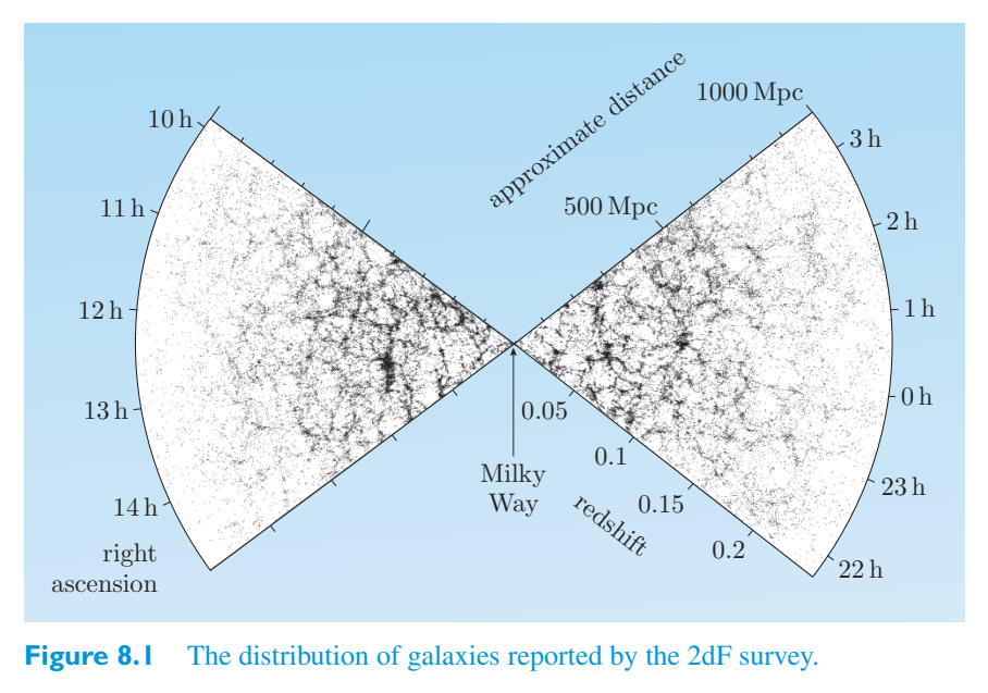
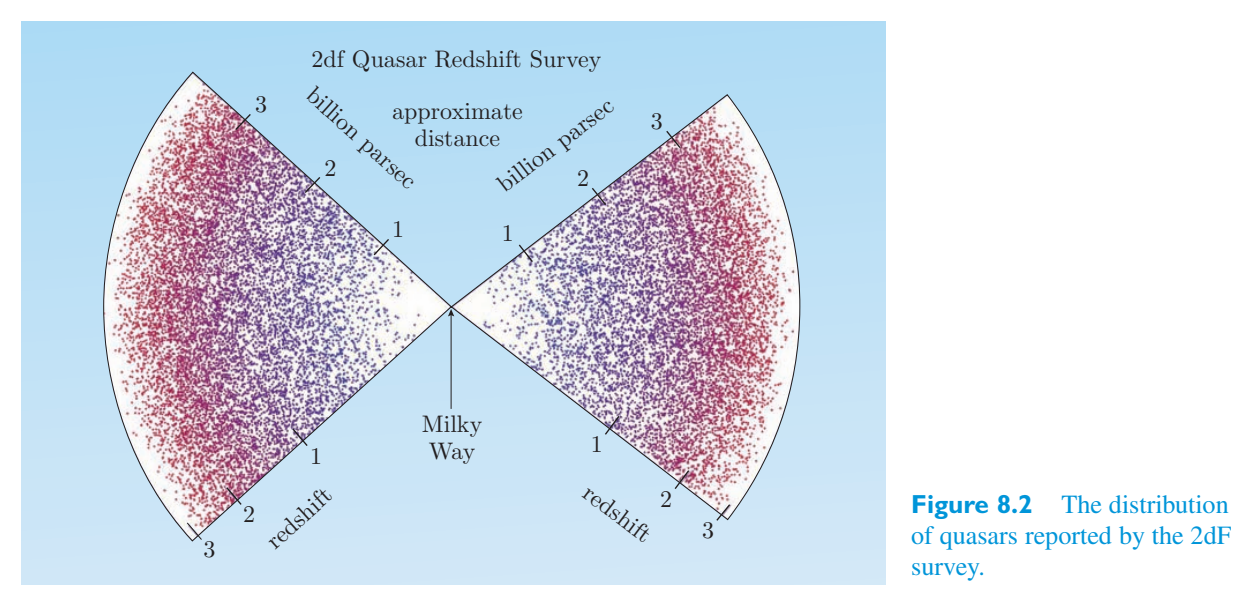
provided by a special part earlier, quasars brightness, thought to by matter falling into a distributed to show the on the large scale they Way. Accepting that isotropic distribution of about all points, and homogeneously at any早先由一个特殊部分提供的类星体亮度,被认为是通过物质落入分布来显示它们在大范围内的走向。接受关于所有点的各向同性分布,并且在任意点均匀分布
Looking at Figure 8.2, the distribution of quasars may not look homogeneous but that is because the distances involved are so vast that the more remote quasars are being seen at significantly earlier epochs in the evolution of the Universe, when the average number of quasars per unit volume was quite different from its current value. The observed distribution of quasars therefore provides evidence of cosmic evolution as well as evidence of isotropy and homogeneity. Although the quasars have always been homogeneously distributed since they first appeared on the cosmic scene, their population is believed to have peaked several billion years ago, hence the peak in the observed number density of quasars at a distance of about 3 billion parsecs.从图 8.2 中可以看出,类星体的分布可能看起来并不均匀,但这是因为所涉及的距离非常遥远,以至于在宇宙演化的早期阶段就可以看到更遥远的类星体,而此时每单位体积的类星体平均数量与当前值有很大不同。因此,观测到的类星体分布提供了宇宙演化的证据以及各向同性和均质性的证据。尽管类星体自首次出现在宇宙场景以来一直是均匀分布的,但据信其数量在数十亿年前达到顶峰,因此观测到的类星体数密度峰值在距离约30亿秒差距处。
A second, even stronger, strand of evidence concerning isotropy comes from observations of the cosmic microwave background radiation (CMBR). This is thermal radiation, meaning that it can be characterized by a temperature, in this case about 2.7 K. The CMBR was discovered in the mid-1960s and has been intensively studied ever since, most recently by the Wilkinson Microwave Anisotropy Probe (WMAP), a specialized space observatory that produced its first results in 2003. The CMBR is believed to have originated in the early Universe and is sometimes popularly described as the ‘echo of the Big Bang’. It is now known to account for the greater part of all the radiant energy in the Universe, and is a major tool for cosmologists in their efforts to understand the Universe.关于各向同性的第二个、甚至更强有力的证据来自对宇宙微波背景辐射(CMBR)的观测。这是热辐射,意味着它可以用温度来表征,在本例中约为 2.7 K。CMBR 于 20 世纪 60 年代中期被发现,此后一直被深入研究,最近由威尔金森微波各向异性探测器 (WMAP) 进行深入研究,这是一个专门的空间天文台,于 2003 年得出了第一个结果。CMBR 被认为起源于早期宇宙,有时被普遍描述为“大爆炸的回声”。现在已知它占宇宙中所有辐射能的大部分,并且是宇宙学家努力了解宇宙的主要工具。
For our present purposes, the most important feature of the CMBR is that, after correcting for the distortions caused by the motion of our observing equipment, it is highly isotropic (see Figure 8.3). The intrinsic mean intensity of the CMBR differs by less than one part in ten thousand in different directions. Since the CMBR is believed to be a universal phenomenon, it can again be argued that the observed isotropy about our location is evidence of isotropy about all locations and is therefore evidence of homogeneity at the present time and, by implication, also evidence of homogeneity at earlier times. It therefore makes good sense to identify the CMBR as a form of ‘background radiation’ since it should be equally prevalent in all parts of space at any given time, unlike starlight, for example, which is associated with localized sources and would therefore be relatively rare in places such as the voids between superclusters.就我们目前的目的而言,CMBR 最重要的特征是,在校正了观测设备运动引起的畸变后,它具有高度各向同性(见图 8.3)。 CMBR 的固有平均强度在不同方向上的差异不到万分之一。由于 CMBR 被认为是一种普遍现象,因此可以再次争论,观察到的关于我们位置的各向同性是所有位置各向同性的证据,因此是当前同质性的证据,并且暗示,也是早期同质性的证据。因此,将 CMBR 识别为“背景辐射”的一种形式是很有意义的,因为它在任何给定时间在空间的所有部分都应该同样普遍,这与星光不同,例如,星光与局部源相关,因此在超星团之间的空隙等地方相对罕见。
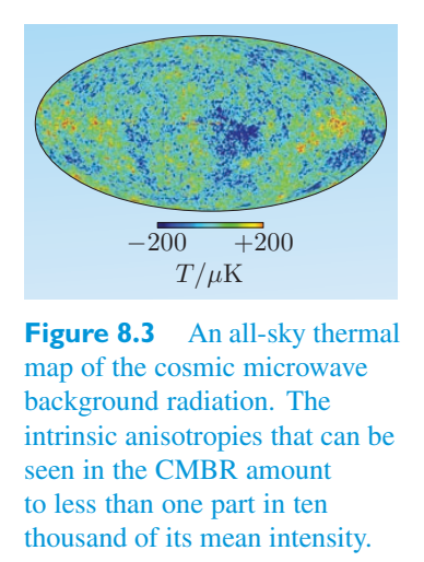
It is worth noting at this point that although isotropy about every point is a sufficient condition to ensure homogeneity, the existence of homogeneity is not sufficient to ensure isotropy. It is quite possible for a distribution to be homogeneous but not isotropic. A uniform magnetic field would be a case in point. The field would have a definite direction at every point, so it would not be isotropic, but provided that it had the same direction at every point, it would be homogeneous. So the assertion that on the large scale the Universe is homogeneous and isotropic has a real and distinctive meaning.此时值得注意的是,虽然每个点的各向同性是保证同质性的充分条件,但同质性的存在并不足以保证各向同性。分布很可能是均匀的但不是各向同性的。均匀磁场就是一个很好的例子。场在每一点都有明确的方向,因此它不会是各向同性的,但如果它在每一点都有相同的方向,它就会是均匀的。因此,在大尺度上宇宙是均匀且各向同性的断言具有真实而独特的意义。
It is significant that the wording of the cosmological principle includes a reference to time, since this leaves open the possibility of cosmic evolution, provided that the evolution is consistent with homogeneity and isotropy. We have already noted the evolution that is thought to have taken place in the population of quasars, but it is also possible for evolution to involve large-scale motion. Observational evidence that the Universe is in fact expanding was published in 1929 by the American astronomer Edwin Hubble (1889–1953). Hubble’s data only extended to relatively nearby galaxies and were complicated by the fact that individual galaxies have their own so-called peculiar motion relative to the large-scale expansion. However, extensive subsequent studies have confirmed that the large-scale motion, sometimes called the Hubble flow, is isotropic so it can be characterized by a single rate of expansion at any time. Since the mid-1990s it has also become clear that the rate of cosmic expansion is currently increasing with time and has been doing so for at least a billion years. As a result we can say not only that the Universe is expanding but also that its expansion is accelerating. The peculiar motions of individual galaxies are generally small and random compared with the overall motion of the Hubble flow. The uniformity of the motion of matter on the large scale provides a third strand of evidence supporting the cosmological principle.值得注意的是,宇宙学原理的措辞包含了对时间的提及,因为这为宇宙演化留下了可能性,只要演化符合同质性和各向同性。我们已经注意到类星体群中发生的演化,但演化也有可能涉及大规模运动。美国天文学家埃德温·哈勃(埃德温·哈勃,1889-1953)于 1929 年发表了宇宙实际上正在膨胀的观测证据。哈勃的数据仅扩展到相对较近的星系,并且由于各个星系相对于大规模膨胀都有自己的所谓奇特运动,因此变得复杂。然而,广泛的后续研究已经证实,大尺度运动(有时称为哈勃流)是各向同性的,因此可以用任何时间的单一膨胀率来表征。自 20 世纪 90 年代中期以来,人们已经清楚地看到,宇宙膨胀的速度目前正在随着时间的推移而增加,并且这种情况已经持续了至少 10 亿年。因此,我们不仅可以说宇宙正在膨胀,而且还可以说它的膨胀正在加速。与哈勃流的整体运动相比,单个星系的奇特运动通常很小且随机。大尺度物质运动的均匀性提供了支持宇宙学原理的第三条证据。
Exercise 8.1 Summarize the three strands of evidence练习 8.1 总结三组证据
that support the cosmological principle.支持宇宙学原理。
8.1.3 Weyl’s postulate8.1.3 外尔假设
Weyl’s postulate was advanced in 1923, by the originator of gauge theory, the mathematical physicist Hermann Weyl (1885–1955). It is essentially an assumption about the matter in the Universe, but it came before the nature and distribution of galaxies was well understood, so Weyl treated the material content of the Universe as a fluid and spoke of its constituent particles as forming a substratum. Modern statements of Weyl’s postulate often replace any mention of the substratum by references to superclusters of galaxies, or even to individual galaxies provided that their peculiar motions are ignored. In this sense, Weyl’s postulate is really an assumption about the nature of the Hubble flow that predates the discovery of that flow.外尔假设由规范理论创始人、数学物理学家赫尔曼·外尔(Hermann Weyl,1885-1955)于 1923 年提出。它本质上是对宇宙中物质的假设,但它是在人们充分理解星系的性质和分布之前提出的,因此外尔将宇宙的物质内容视为流体,并将其组成粒子视为形成基质。外尔假设的现代陈述经常用超星系团来代替对底层的任何提及,甚至是单个星系,只要它们的特殊运动被忽略。从这个意义上说,外尔假设实际上是对哈勃流性质的假设,该假设早于哈勃流的发现。
From a modern perspective the significance of Weyl’s postulate is that it recognizes the existence of a privileged class of observers who have a particularly simple view of the Universe. These are the observers who move with the Hubble flow. You can think of each such observer as moving with their local supercluster or even with their own local galaxy, as long as its peculiar motion is ignored. It is these observers, sometimes called fundamental observers, who will find that the Universe around them (including the CMBR) is isotropic. A non-fundamental observer who moves relative to the local fundamental observer would not find that the Universe was expanding uniformly in all directions, nor would such a non-fundamental observer find the CMBR to be isotropic. In terms of fundamental observers, Weyl’s postulate can be stated as follows.从现代的角度来看,外尔假设的意义在于它承认存在一个特权观察者阶层,他们对宇宙有着特别简单的看法。这些是随哈勃流移动的观察者。您可以将每个这样的观察者视为与当地超星系团一起移动,甚至与当地星系一起移动,只要忽略其特殊的运动即可。正是这些观察者(有时称为基本观察者)会发现他们周围的宇宙(包括 CMBR)是各向同性的。相对于局部基本观察者移动的非基本观察者不会发现宇宙在所有方向上均匀膨胀,这样的非基本观察者也不会发现 CMBR 是各向同性的。就基本观察者而言,外尔假设可以表述如下。
Weyl’s postulate外尔假设
In cosmic spacetime there exists a set of privileged fundamental observers whose world-lines form a smooth bundle of time-like geodesics. These geodesics never meet at any event, apart perhaps from an initial singularity in the past and/or a final singularity in the future.在宇宙时空中,存在着一组享有特权的基本观察者,他们的世界线形成了一束光滑的类时间测地线。这些测地线在任何情况下都不会相遇,除了过去的初始奇点和/或未来的最终奇点之外。
The implications of Weyl’s postulate are indicated in Figure 8.4. Essentially, the postulate supposes that the Universe is structured and evolves in a sufficiently orderly way that the proper time measured by each fundamental observer can be correlated with that of every other fundamental observer so that a value of a single, universally meaningful cosmic time can be associated with every event.外尔假设的含义如图 8.4 所示。从本质上讲,该假设假设宇宙以足够有序的方式构建和演化,每个基本观察者测量的正确时间可以与其他每个基本观察者的正确时间相关联,以便单个、具有普遍意义的宇宙时间的值可以与每个事件相关联。
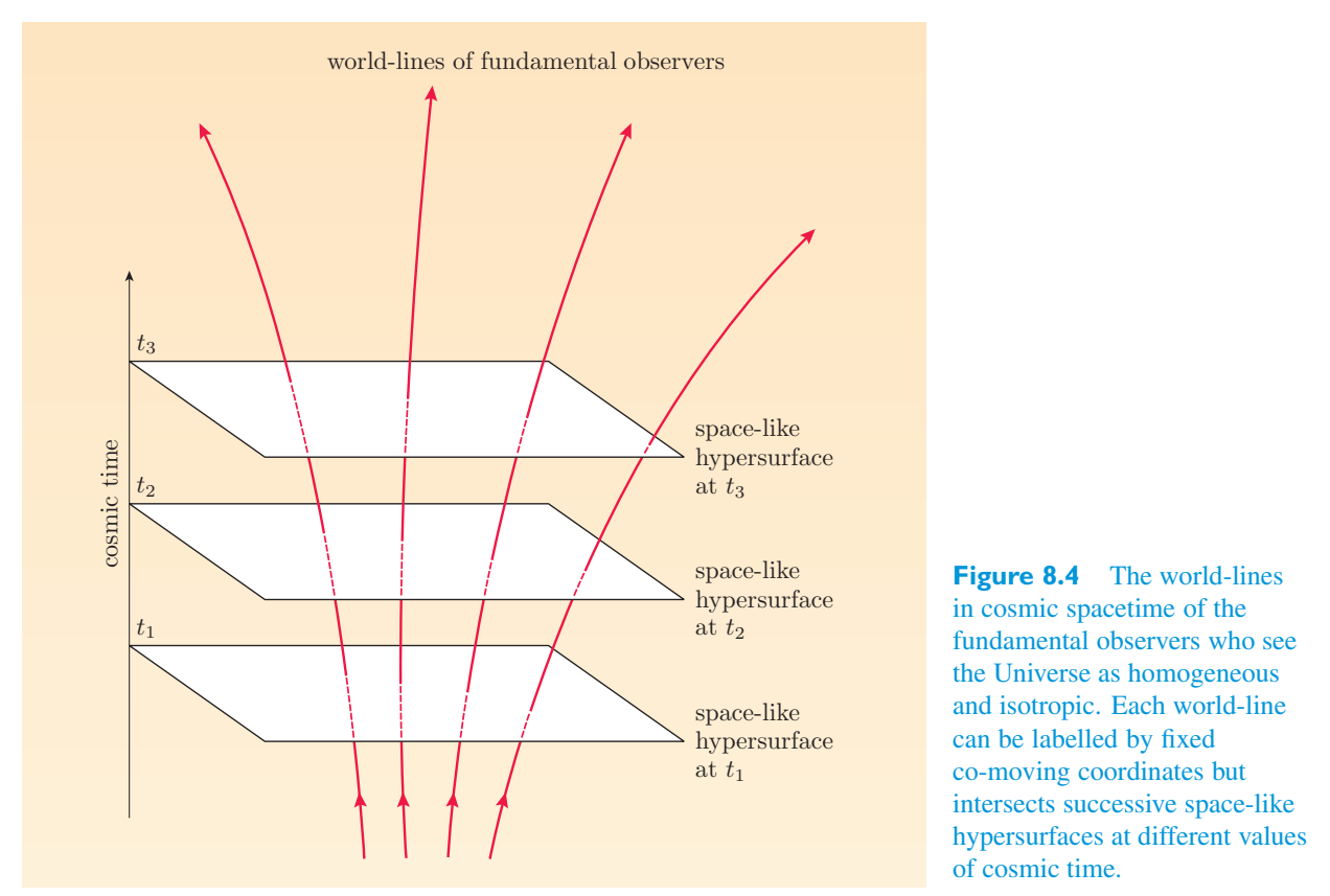
This might be done, for example, by all fundamental observers agreeing to use the proper time since the Big Bang or, more realistically, the proper time since the CMBR had some particular mean intensity. The ability to define a cosmic time means that we can identify all the events characterized by any particular value of cosmic time. Such a set of events will form a three-dimensional space, technically referred to as a space-like hypersurface with geometric properties that are homogeneous and isotropic. Each of the ‘surfaces’ in Figure例如,这可以通过所有基本观察者同意使用自大爆炸以来的固有时间,或者更现实地,自 CMBR 具有某种特定平均强度以来的固有时间来完成。定义宇宙时间的能力意味着我们可以识别以任何特定宇宙时间值为特征的所有事件。这样的一组事件将形成一个三维空间,技术上称为类空间超曲面,具有均匀且各向同性的几何特性。图中的每个“表面”
8.4 represents one of8.4 代表其中之一
these space-like hypersurfaces and can be thought of as the whole of space at a particular moment of cosmic time. The lines threading the surfaces represent the world-lines of the fundamental observers, and may only diverge or converge in such a way that overall homogeneity and isotropy are preserved throughout cosmic time.这些类似空间的超曲面,可以被认为是宇宙时间特定时刻的整个空间。穿过表面的线代表基本观察者的世界线,并且只能以在整个宇宙时间内保持整体均匀性和各向同性的方式发散或汇聚。
Each of the fundamental observer world-lines in Figure图中每个基本观察者世界线
8.4 may be characterized8.4 可表征
coordinates, \(x^1\), \(x_{2}\) on any particular space-like hypersurface by three spatial and \(x^{3}\). Remembering that coordinates have no immediate metrical significance in general relativity, we may, if we wish, choose to define our coordinate system in such a way that the world-line of a fundamental observer is assigned the same values of the three spatial coordinates on every space-like hypersurface. Coordinates of this kind are widely used in cosmology and are called co-moving coordinates. In an expanding (or contracting) Universe, the grid of co-moving coordinates must expand or contract with the space-like hypersurfaces. So, in our Universe, a co-moving coordinate grid, like the fundamental observers, must ‘go with the flow’. It follows that if we ignore the individual peculiar motions, then every galaxy will have constant co-moving coordinates. The behaviour of co-moving coordinates in an expanding Universe is indicated in Figure 8.5.坐标,\(x^1\),\(x_{2}\) 在任何特定的类空间超曲面上由三个空间和 \(x^{3}\) 组成。请记住,坐标在广义相对论中没有直接的度规意义,如果我们愿意,我们可以选择以这样的方式定义我们的坐标系,即为基本观察者的世界线分配每个类空间超曲面上三个空间坐标的相同值。这种坐标在宇宙学中被广泛使用,被称为共动坐标。在膨胀(或收缩)的宇宙中,共动坐标网格必须随类空间超曲面膨胀或收缩。因此,在我们的宇宙中,一个共动的坐标网格,就像基本观察者一样,必须“顺其自然”。由此可见,如果我们忽略个体的特殊运动,那么每个星系都将具有恒定的共动坐标。图 8.5 显示了膨胀宇宙中坐标共动的行为。
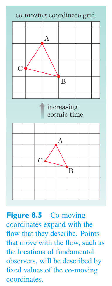
We ourselves, living on the Earth and orbiting the Sun, are almost in the situation of fundamental observers. The Milky Way has some peculiar motion relative to the frame of a local fundamental observer, and we also participate in the motion of the Sun relative to the centre of the Milky Way and the motion of the Earth as it orbits the Sun. It is for this reason that we said in the previous subsection that the CMBR was highly isotropic after correcting for the distortions caused by the motion of our observing equipment. In fact, observations of a large-scale anisotropy in the CMBR, called the dipole anisotropy (see Figure 8.6), allow us to work out our motion relative to the frame of the local fundamental observer. The results show that in such a frame, the Sun is travelling at about a thousandth of the speed of light in the direction of the constellation of Leo. (The precise figures are 368 ± 2 \(\mathrm{km\,s^{-1}}\) towards the point with right ascension 11 h 22 min and declination − 7.22 degrees.) The orbital speed of the Earth relative to the Sun is only about one twelfth of the Sun’s speed, so it can be ignored for most practical purposes.我们生活在地球上并绕太阳运行,几乎处于基本观察者的境地。银河系相对于当地基本观测者的坐标系有一些特殊的运动,我们也参与了太阳相对于银河系中心的运动以及地球绕太阳运行的运动。正是由于这个原因,我们在上一小节中说过,在校正了我们观测设备运动引起的畸变后,CMBR 具有高度各向同性。事实上,对 CMBR 中大尺度各向异性(称为偶极子各向异性)的观测(见图 8.6)使我们能够计算出相对于局部基本观察者坐标系的运动。结果表明,在这样的框架中,太阳正以大约千分之一光速朝狮子座方向行进。 (精确的数字是 368 ± 2 \(\mathrm{km\,s^{-1}}\) 到赤经 11 小时 22 分钟、赤纬 − 7.22 度的点。)地球相对于太阳的轨道速度大约仅为太阳速度的十二分之一,因此在大多数实际用途中可以忽略不计。
In what follows it will be convenient to regard every fundamental observer as being located in a galaxy that exactly follow the isotropic Hubble flow. This amounts to ignoring the peculiar motions that galaxies actually possess.在下文中,可以方便地将每个基本观察者视为位于完全遵循各向同性哈勃流的星系中。这相当于忽略了星系实际拥有的特殊运动。
8.2 Robertson–Walker spacetime8.2 罗伯逊-沃克时空
Cosmologists have developed, investigated and classified a wide range of relativistic cosmological models, including some that are neither homogeneous nor isotropic. However, the overwhelming majority of the investigations have concerned models that are homogeneous and isotropic, and therefore conform to the requirements of the cosmological principle. Around 1935, Howard Robertson (1903–1961) of the California Institute of Technology and Arthur Walker (1909–2001) of the University of Liverpool showed, independently, that a single spacetime metric underlies all relativistic models that are homogeneous and isotropic. That metric is now known as the Robertson–Walker metric. The Robertson–Walker metric and the spacetime that it describes are the subject of this section.宇宙学家已经开发、研究和分类了广泛的相对论宇宙学模型,其中包括一些既不是均匀的也不是各向同性的模型。然而,绝大多数研究都涉及均匀且各向同性的模型,因此符合宇宙学原理的要求。1935 年左右,加州理工学院的霍华德·罗伯逊(Howard Robertson,1903-1961)和利物浦大学的阿瑟·沃克(Arthur Walker,1909-2001)独立地表明,单一时空度规是所有同质和各向同性相对论模型的基础。该度规现在被称为罗伯逊-沃克指标。罗伯逊-沃克度规及其描述的时空是本节的主题。
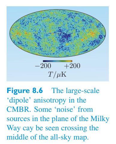
8.2.1 The Robertson–Walker metric8.2.1 罗伯逊-沃克度规
Based on the three principles introduced in the previous section, it is natural for a fundamental observer to describe cosmic spacetime using a squared line element of the form基于上一节介绍的三个原理,基本观察者很自然地使用以下形式的平方线元素来描述宇宙时空
where \(t\) represents cosmic time, \(x^1\), \(x^2\) and \(x^3\) are co-moving coordinates, and the metric coefficients \(g_{ij}\) are functions of \(t\), \(x^1\), \(x^2\) and \(x^3\).其中 \(t\) 表示宇宙时间,\(x^1\)、\(x^2\) 和 \(x^3\) 是共动坐标,度规系数 \(g_{ij}\) 是 \(t\)、\(x^1\)、\(x^2\) 和 \(x^3\) 的函数。
Spatial homogeneity and isotropy require that the ratios of distances are the same at all times. So three fundamental observers located at the corners of a triangle at some cosmic time \(t_1\), will also be at the corners of a similar triangle at cosmic time \(t_2\). The triangle may be bigger or smaller, but its angles will be the same, and each side will have increased or decreased its length by the same factor. We can incorporate this requirement into the metric by insisting that the cosmic time enters the metric coefficients \(g_{ij}\) only through a common scaling function. For later convenience we shall write this common function as \(S^2(t)\), so空间均匀性和各向同性要求距离之比在所有时刻都相同。因此,在某个宇宙时间 \(t_1\) 位于三角形三个顶点上的三个基本观察者,在宇宙时间 \(t_2\) 也将位于一个相似三角形的三个顶点上。三角形可以变大或变小,但角度保持不变,每条边的长度都按同一因子增加或减少。我们可以要求宇宙时间只通过一个共同的尺度函数进入度规系数 \(g_{ij}\),从而把这一要求写进度规。为方便起见,我们把这个共同函数写成 \(S^2(t)\),于是
where each of the coefficients \(h_{ij}=g_{ij}/S^2(t)\) depends only on \(x^1\), \(x^2\) and \(x^3\).其中每个系数 \(h_{ij}=g_{ij}/S^2(t)\) 只依赖于 \(x^1\)、\(x^2\) 和 \(x^3\)。
Now, the curvature tensor of a three-dimensional space generally has \(3^4=81\) components, of which 6 are independent. However, since the space described by \(h_{ij}\) is homogeneous and isotropic, the curvature must be the same everywhere and in all directions. As a result, the curvature must be fixed by a single parameter. If the properties of the space are also independent of time, then that single parameter must be a constant. We shall denote that constant by the upper-case letter \(K\). The metric that describes a three-dimensional space of constant curvature is well known to mathematicians. If we use its most common form to replace the coefficients \(h_{ij}\) in Equation 8.6, we obtain the metric三维空间的曲率张量一般有 \(3^4=81\) 个分量,其中 6 个是独立的。然而,由于 \(h_{ij}\) 所描述的空间是均匀且各向同性的,曲率必须在所有位置和所有方向上都相同。因此,曲率必须由一个单独的参数固定。如果空间性质还与时间无关,那么这个单独参数就必须是常数。我们用大写字母 \(K\) 表示这个常数。描述三维常曲率空间的度规是数学家熟知的。若用其最常见形式替换方程 8.6 中的系数 \(h_{ij}\),就得到度规
where we have replaced the general co-moving coordinates \(x^1\), \(x^2\), \(x^3\) by the co-moving polar coordinates \(r\), \(\theta\), \(\phi\). You will see why we have called the radial coordinate \(r\) in just a moment. First, though, note that the expression inside the square brackets represents a space of constant curvature. Its Riemann curvature components are \(R^{ij}{}_{kl}=K(h^i{}_k h^j{}_l-h^i{}_l h^j{}_k)\), the Ricci tensor components are \(R^{ij}=-2K h^{ij}\), and the Ricci curvature scalar is \(R=-6K\). For simplicity, such a space is said to have curvature \(K\). The effect of multiplying the expression in square brackets by \(S^2(t)\) is to produce a rescaled version of the space that at time \(t\) has curvature \(K/S^2(t)\). (This is rather like the effect of inflating a spherical balloon, where increasing the balloon’s radius by a factor of 2 will make the surface flatter, reducing the (Gaussian) curvature by a factor of 4.)这里我们已把一般共动坐标 \(x^1\)、\(x^2\)、\(x^3\) 换成共动极坐标 \(r\)、\(\theta\)、\(\phi\)。稍后你会看到为什么把径向坐标记为 \(r\)。不过首先要注意,方括号中的表达式表示一个常曲率空间。它的黎曼曲率分量为 \(R^{ij}{}_{kl}=K(h^i{}_k h^j{}_l-h^i{}_l h^j{}_k)\),Ricci 张量分量为 \(R^{ij}=-2K h^{ij}\),Ricci 曲率标量为 \(R=-6K\)。为简明起见,这样的空间称为具有曲率 \(K\)。把方括号中的表达式乘以 \(S^2(t)\) 的效果,是得到一个重新缩放的空间;在时间 \(t\),它的曲率为 \(K/S^2(t)\)。(这很像给球形气球充气:若气球半径增加 2 倍,表面会更平坦,高斯曲率会减小 4 倍。)
Equation 8.7 is one form of the Robertson–Walker metric, but not the most common form. It turns out that for many purposes the value of the curvature constant K is less important than whether it is positive or negative. Consequently it is generally convenient to carry out a coordinate transformation that has the effect of replacing the spatial curvature K by a related quantity k, called the curvature parameter, that can take only the values +1, 0 or − 1. This can be achieved by introducing a new rescaled radial coordinate公式 8.7 是罗伯逊-沃克度规的一种形式,但不是最常见的形式。事实证明,对于许多目的来说,曲率常数 K 的值并不重要,重要的是它是正还是负。因此,通常可以方便地执行坐标变换,将空间曲率 K 替换为相关量 k(称为曲率参数),该量只能取值 +1、0 或 - 1。这可以通过引入新的重新缩放的径向坐标来实现
Using this to eliminate all occurrences of r in Equation用它来消除方程中所有出现的 r
8.7, we can rewrite the8.7,我们可以重写
Robertson–Walker metric in its most common form.罗伯逊-沃克度规最常见的形式。
The Robertson–Walker metric罗伯逊-沃克度规
Here \(r\), \(\theta\), \(\phi\) are still co-moving coordinates (the rescaling doesn’t change that) and the information about distance ratios at different times is now contained in the time-dependent function \(R(t)\), which is therefore known as the scale factor and is defined by the relation这里 \(r\)、\(\theta\)、\(\phi\) 仍然是共动坐标(重新缩放不会改变这一点),不同时刻的距离比例信息现在包含在随时间变化的函数 \(R(t)\) 中;因此 \(R(t)\) 称为尺度因子,并由下式定义
It is important to note that this scale factor \(R(t)\) is quite distinct from the Ricci scalar that appears in the field equations and which is also denoted by R. From here on, R will always be the scale factor, never the Ricci scalar.值得注意的是,这个尺度因子 \(R(t)\) 与出现在场方程中且也用 R 表示的 Ricci 标量完全不同。从这里开始,R 将始终是尺度因子,而不是 Ricci 标量。
If the scale factor \(R(t)\) increases with time, then the fundamental observers become more widely separated with time, the galaxies containing those fundamental observers get further apart, and the Universe is said to be expanding. If \(R(t)\) decreases with time, then the fundamental observers and their associated galaxies get closer together, and the Universe may be said to be contracting. Remember, though, that throughout this process the co-moving coordinates of any fundamental observer remain fixed at all times. Also remember that the space-like hypersurfaces are homogeneous and isotropic, so although the coordinate system will have some particular origin and some particular orientation, any point may be chosen to be the origin, and the chosen orientation of the axes is equally arbitrary.如果尺度因子 \(R(t)\) 随着时间的推移而增加,那么基本观察者随着时间的推移会变得更加分离,包含这些基本观察者的星系也会变得更加分离,并且宇宙被认为正在膨胀。如果 \(R(t)\) 随着时间的推移而减小,那么基本观测者及其相关星系就会靠得更近,宇宙可以说是在收缩。但请记住,在整个过程中,任何基本观察者的共动坐标始终保持固定。还要记住,类空间超曲面是均匀且各向同性的,因此尽管坐标系将具有某些特定的原点和某些特定的方向,但可以选择任何点作为原点,并且所选择的轴方向同样是任意的。
As a result of the rescaling, the curvature of the constant-\(t\) space-like hypersurface will be \(k/R^2(t)\).重新缩放后,常 \(t\) 类空间超曲面的曲率为 \(k/R^2(t)\)。
Apart from the cosmic time and the co-moving coordinates, the scale factor \(R(t)\) and the curvature parameter \(k\) are the only quantities that appear in the Robertson–Walker metric. Both are important. The rest of this section will be mainly concerned with the significance of \(k\); the role of \(R(t)\) will feature prominently in Section 8.3.除了宇宙时间和共动坐标之外,尺度因子 \(R(t)\) 与曲率参数 \(k\) 是罗伯逊-沃克度规中出现的仅有两个量。二者都很重要。本节余下部分主要讨论 \(k\) 的意义;\(R(t)\) 的作用将在第 8.3 节中占据核心位置。
8.2.2 Proper distances and velocities in cosmic spacetime8.2.2 宇宙时空中的固有距离和速度
We already know that in the Robertson–Walker metric, \(t\) represents the cosmic time, which can be related to the proper time measured by any fundamental observer. This is the time that might be measured on a clock carried by the fundamental observer. However, we still don’t know the precise relationship between the fixed co-moving coordinates of two points and the proper distance that would be measured between those points by connecting them with a line of stationary measuring rods at some particular time \(t\).我们已经知道,在罗伯逊-沃克度规中,\(t\) 表示宇宙时间,它可以与任何基本观察者测得的固有时间联系起来。这就是基本观察者随身携带的时钟会测得的时间。然而,我们仍然不知道两个点的固定共动坐标,与在某个特定时间 \(t\) 用一排静止测量杆连接两点时测得的固有距离之间的精确关系。
- ● Assuming that the measuring rods can be laid along the shortest path between假设测量杆可以沿着最短路径铺设
the two points, how would you describe that path?这两点,你会如何描述这条道路?
❍ The path of shortest length between two points at a given time would lie in a particular space-like hypersurface, and would be a geodesic of that hypersurface.❍ 给定时间两点之间的最短路径将位于特定的类似空间的超曲面中,并且将是该超曲面的测地线。
For two simultaneous events that occur with infinitesimally separated positions, \((r,\theta,\phi)\) and \((r+dr,\theta+d\theta,\phi+d\phi)\), the proper distance separating them can be read directly from the Robertson–Walker line element. Using the symbol \(d\sigma\) to represent that infinitesimal distance, we have对于两个同时发生、位置相差无穷小的事件,坐标分别为 \((r,\theta,\phi)\) 和 \((r+dr,\theta+d\theta,\phi+d\phi)\),它们之间的固有距离可以直接从罗伯逊-沃克线元读出。用符号 \(d\sigma\) 表示这个无穷小距离,有
Note that this proper distance element depends on the proper time at which it is measured. This is to be expected in an expanding or contracting Universe since proper separations will change with time even though (co-moving) coordinates don’t change their values.请注意,该固有距离元素取决于测量它的固有时间。这在膨胀或收缩的宇宙中是可以预料的,因为即使(共动)坐标不改变它们的值,适当的分离也会随着时间而改变。
When dealing with finite separations, the problem of working out proper distances is generally quite challenging. It involves integrating the distance element given in Equation 8.11 along a pathway, and this usually requires the introduction of parameters, just as we did in Chapter 3. However, the problem can be greatly simplified by making use of the homogeneity of the space-like hypersurfaces. Given two points on such a hypersurface, we can always choose one of them to be the origin of coordinates. The other will then be at some specific co-moving radial coordinate value, \(r=\chi\) say, in a fixed direction, specified by particular values of \(\theta\) and \(\phi\). In such a case, the two points are linked by a purely radial path that will always be a geodesic (we shall not prove this). Along that radial path \(d\theta=0\) and \(d\phi=0\), so the element of proper distance is just \(d\sigma=R(t)\,dr/(1-kr^2)^{1/2}\). Thus, given two points separated by a fixed radial co-moving coordinate \(\chi\), the proper distance between them at time \(t\) will be处理有限距离时,求固有距离通常相当困难。它需要沿路径对方程 8.11 给出的距离元积分,通常还需要像第 3 章那样引入参数。不过,利用类空间超曲面的均匀性,可以大大简化问题。给定这样一个超曲面上的两个点,我们总可以选择其中一个作为坐标原点。另一个点就在某个特定的共动径向坐标值处,记为 \(r=\chi\),方向固定,并由特定的 \(\theta\) 和 \(\phi\) 值指定。在这种情况下,这两个点由一条纯径向路径连接,而这条路径总是一条测地线(这里不证明)。沿这条径向路径有 \(d\theta=0\) 且 \(d\phi=0\),所以固有距离元就是 \(d\sigma=R(t)\,dr/(1-kr^2)^{1/2}\)。因此,给定由固定径向共动坐标 \(\chi\) 分隔的两点,它们在时间 \(t\) 的固有距离为
Whether k is +1, 0 or − 1, this is a standard integral with a well-known result.无论k是+1、0还是−1,这都是具有众所周知结果的标准积分。
These three relationships are illustrated in Figure 8.7.这三种关系如图 8.7 所示。
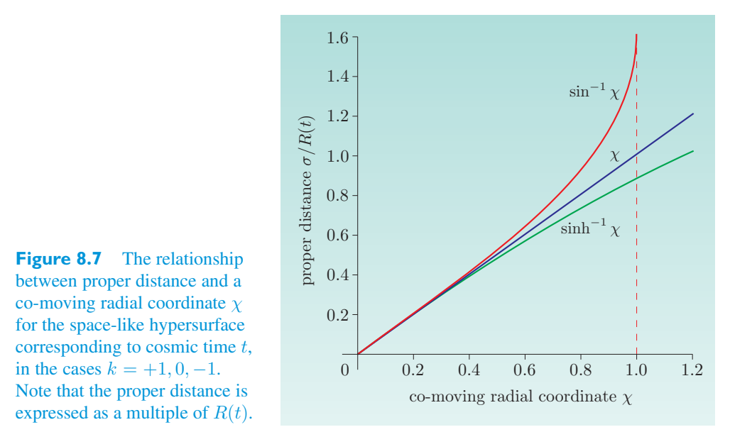
All three of these functions behave in a similar way for small values of \(\chi\), but as \(\chi\) increases, they start to separate until the value \(\chi=1\) is reached, at which point \(\sin^{-1}\chi\) diverges. These differences are, of course, a result of the intrinsic curvature of the space-like hypersurfaces. We shall explore this more fully in the next subsection.对于较小的 \(\chi\),这三个函数的行为相似;但随着 \(\chi\) 增大,它们开始分离,直到达到 \(\chi=1\),此时 \(\sin^{-1}\chi\) 发散。当然,这些差异来自类空间超曲面的内禀曲率。下一小节会更充分地讨论这一点。
An important point to note concerning co-moving coordinates and their relationship to proper distances involves units and dimensions. The proper distance between two points must be a length. However, the co-moving coordinate is not subject to the same restriction. Since all proper lengths are proportional to the scale factor \(R(t)\), it is conventional to treat the co-moving coordinate \(r=\chi\) as dimensionless and the scale factor \(R(t)\) as having the dimensions of length.关于共动坐标及其与固有距离的关系,有一点涉及单位和量纲,值得注意。两点之间的固有距离必须具有长度量纲。然而,共动坐标不受同样限制。由于所有固有长度都正比于尺度因子 \(R(t)\),通常把共动坐标 \(r=\chi\) 视为无量纲量,而把尺度因子 \(R(t)\) 视为具有长度量纲。
Though we now have an expression for proper distance, it will be of interest only for certain theoretical purposes. It’s not a distance that can be directly observed astronomically; we can’t really set up lines of stationary rulers stretching from one galaxy to another. Nonetheless, it is interesting to ask how quickly the proper distance between fundamental observers would change as a result of any uniform expansion or contraction. (We have to ask about the proper distance since the co-moving coordinate \(\chi\) won’t change at all.) Defining the proper radial velocity as the rate of change of proper distance with respect to cosmic time, we see from the above that尽管我们现在有了固有距离的表达式,但它仅对某些理论目的有意义。这不是天文上可以直接观测到的距离;我们无法真正建立从一个星系延伸到另一个星系的固定标尺线。尽管如此,有趣的是,由于任何均匀的膨胀或收缩,基本观察者之间的固有距离会以多快的速度发生变化。(我们必须问固有距离,因为共动坐标 \(\chi\) 根本不会改变。)将适当的视向速度定义为固有距离相对于宇宙时间的变化率,从上面我们可以看出
In each case we can replace the term involving \(\chi\) by \(\sigma/R\). This leads to the same expression for the proper velocity in all three cases:在每种情况下,都可以把含有 \(\chi\) 的项替换为 \(\sigma/R\)。这使三种情况下的固有速度都具有同一个表达式:
It is conventional to write this relationship in the more memorable form按照惯例,以更容易记住的形式来写这种关系
where \(d_p\) represents the proper distance between two fundamental observers or their galaxies, \(v_p\) represents the proper radial velocity at which they are separating (for positive \(v_p\)) or coming together (for negative \(v_p\)), and \(H(t)\), which is called the Hubble parameter, is defined as follows.其中 \(d_p\) 表示两个基本观察者或其星系之间的固有距离,\(v_p\) 表示它们相互远离(\(v_p>0\))或相互接近(\(v_p<0\))时的固有径向速度,\(H(t)\) 称为哈勃参数,定义如下。
The Hubble parameter哈勃参数
Equation 8.16 tells us that at any cosmic time \(t\), every fundamental observer is moving radially relative to every other fundamental observer at a proper speed that is proportional to the proper distance that separates them. Note that this is an exact consequence of the nature of Robertson–Walker spacetime. Later we shall re-examine this result in connection with Hubble’s observations of cosmic expansion. At that stage we shall relate the proper distance to some other distances that really can be measured and also relate the Hubble parameter to an observable quantity known as the Hubble constant.方程 8.16 告诉我们,在任意宇宙时间 \(t\),每个基本观察者相对于其他每个基本观察者都以某个固有速度径向运动,而这个速度正比于二者之间的固有距离。注意,这是罗伯逊-沃克时空性质的严格结果。稍后我们会结合哈勃对宇宙膨胀的观测重新考察这个结果。那时我们会把固有距离与一些真正可测的其他距离联系起来,并把哈勃参数与称为哈勃常数的可观测量联系起来。
Exercise 8.2 It was claimed above that at any fixed time, a radial line through练习8.2 上面声称在任何固定时间,一条径向线穿过
the origin of a Robertson–Walker spacetime would be a geodesic of the relevant three-dimensional space-like hypersurface. Outline the procedure that you would follow to establish the truth of this claim, starting from the Robertson–Walker metric.罗伯逊-沃克时空的起源将是相关三维类空间超曲面的测地线。概述从罗伯逊-沃克度规开始,您将遵循的确定此主张真实性的程序。
8.2.3 The cosmic geometry of space and spacetime8.2.3 空间和时空的宇宙几何
In general, a homogeneous and isotropic space-like hypersurface has no centre and no boundary. (Do not mistake the point arbitrarily chosen to be the origin of coordinates with a physically significant centre point.) However, such a hypersurface can have a curvature and can be characterized by a curvature parameter \(k\). In what follows we shall consider the geometrical significance of some particular choices of \(k\) and \(R(t)\). Remember throughout that \(k\) is the curvature parameter, not the curvature. As noted earlier, the curvature of any fixed-\(t\) space-like hypersurface is given by \(k/R^2(t)\).一般而言,均匀且各向同性的类空间超曲面没有中心,也没有边界。(不要把任意选作坐标原点的点误认为物理上特殊的中心点。)不过,这样的超曲面可以有曲率,并可由曲率参数 \(k\) 表征。下面我们将考虑若干特定 \(k\) 和 \(R(t)\) 选择的几何意义。始终要记住,\(k\) 是曲率参数,不是曲率本身。如前所述,任何固定 \(t\) 的类空间超曲面的曲率为 \(k/R^2(t)\)。
Case 1: \(k = 0\) and \(R(t)\) = constant情况 1:\(k = 0\) 和 \(R(t)\) = 常量
In this case the constant scale factor can be absorbed into a rescaled radial coordinate with the result that the Robertson–Walker line element of Equation 8.9 reduces to the Minkowski metric of Chapter 3 expressed in spherical coordinates:在这种情况下,常数尺度因子可以被吸收到重新调整比例的径向坐标中,结果是方程 8.9 的罗伯逊-沃克线元素简化为第 3 章中用球坐标表示的闵可夫斯基度规:
Each space-like hypersurface (representing space at some particular cosmic time t) will have the geometry of a three-dimensional space with zero curvature (i.e. Euclidean 3 -space), and the co-moving coordinate grid will neither expand nor contract. Each fundamental observer would be at rest relative to every other fundamental observer, and each would find that there was no gravity and that special relativity applied everywhere. In this case the Riemann curvature tensor will be zero everywhere and at all times. In short, space would be flat at all times, and the Robertson–Walker spacetime would also be flat.每个类空间超曲面(代表某个特定宇宙时间 t 的空间)将具有曲率为零的三维空间(即欧几里得 3 空间)的几何形状,并且共动坐标网格既不会膨胀也不会收缩。每个基本观察者都会相对于其他每个基本观察者处于静止状态,并且每个基本观察者都会发现不存在引力并且狭义相对论无处不在。在这种情况下,黎曼曲率张量在任何地方、任何时候都为零。简而言之,空间在任何时候都是平坦的,罗伯逊-沃克时空也都是平坦的。
To be consistent with general relativity, the field equations would demand that this gravity-free, flat spacetime contained no matter, radiation or dark energy, so this really isn’t an interesting case from a physical point of view. Nonetheless, it’s interesting to see that Minkowski spacetime can emerge as a limiting case of Robertson–Walker spacetime.为了与广义相对论保持一致,场方程要求这个无引力、平坦的时空不包含物质、辐射或暗能量,所以从物理角度来看,这确实不是一个有趣的情况。尽管如此,有趣的是,闵可夫斯基时空可以作为罗伯逊-沃克时空的极限情况出现。
Case 2: \(k = 0\) and \(R^3(t)\) = constant情况 2:\(k = 0\),且 \(R^3(t)\) 为常数
In this case the three-dimensional space-like hypersurfaces will again have the zero-curvature geometry of Euclidean 3 -space. The internal angles of a triangle add up to \(\pi\) radians, and the ratio of the circumference of a circle to its radius will be 2 \(\pi\). As we saw in the previous subsection, another indication of the spatial flatness is the proportionality between the co-moving radial coordinate \(\chi\) and the proper distance \(\sigma\) at any fixed value of t:在这种情况下,三维类空间超曲面将再次具有欧几里得 3 空间的零曲率几何形状。三角形的内角之和为 \(\pi\) 弧度,圆的周长与其半径之比为 2 \(\pi\)。正如我们在上一小节中看到的,空间平坦度的另一个指标是在任何固定 t 值时,共动径向坐标 \(\chi\) 与固有距离 \(\sigma\) 之间的比例:
\(\sigma(t)=R(t)\chi\) if \(k = 0\).若 \(k = 0\),则 \(\sigma(t)=R(t)\chi\)。
However, the full four-dimensional Robertson–Walker spacetime will not be flat because the scale factor \(R(t)\) will cause the distance between co-moving locations to change, and this will generally prevent the Riemann curvature tensor from vanishing.然而,完整的四维罗伯逊-沃克时空不会是平坦的,因为尺度因子 \(R(t)\) 会导致共动位置之间的距离发生变化,这通常会阻止黎曼曲率张量消失。
Exercise 8.3 ‘The metric used in special relativity is练习 8.3 狭义相对论中使用的度规是
a particular case of the Robertson–Walker metric for which \(k = 0\), i.e. for which space is flat.’ Comment on the accuracy of this statement.罗伯逊-沃克度规的一个特殊情况,其中 \(k = 0\),即空间是平坦的。”对此陈述的准确性发表评论。
Case 3: \(k = +1\) and \(R^3(t)\) = constant情况 3:\(k = +1\),且 \(R^3(t)\) 为常数
In this case both four-dimensional Robertson–Walker spacetime and its three-dimensional space-like hypersurfaces will have a curved geometry. We have already seen that on any particular hypersurface, the proper distance from the origin is related to the radial co-moving coordinate \(r=\chi\) by \(\sigma(t)=R(t)\sin^{-1}\chi\), so \(\sigma\) increases more rapidly with increasing \(\chi\) than in a flat space. Using the proper distance element of Equation 8.11 and the parameterized path method of Chapter 3, an integral around a circle of co-moving coordinate radius \(\chi\), centred on the origin and located in the \(\theta=\pi/2\) plane for simplicity, shows that the circle has proper circumference \(2\pi R(t)\chi\). It follows that the ratio of proper circumference to proper radius for such a circle is在这种情况下,四维罗伯逊-沃克时空及其三维类空间超曲面都具有弯曲几何。我们已经看到,在任一给定超曲面上,从原点出发的固有距离与径向共动坐标 \(r=\chi\) 的关系为 \(\sigma(t)=R(t)\sin^{-1}\chi\),因此 \(\sigma\) 随 \(\chi\) 增大得比平直空间中更快。使用方程 8.11 的固有距离元和第 3 章的参数化路径方法,沿一个以原点为中心、为简单起见位于 \(\theta=\pi/2\) 平面内、共动坐标半径为 \(\chi\) 的圆积分,可得该圆的固有周长为 \(2\pi R(t)\chi\)。因此,这样一个圆的固有周长与固有半径之比为
proper circumference of circle proper radius圆的固有周长、固有半径
We have also seen that the proper distance diverges as \(\chi\) approaches 1.我们还看到,当 \(\chi\) 接近 1 时,固有距离会发散。
All these properties are indications of the positive curvature of the hypersurface. The effects produced are easily remembered by looking at the \(k = +1\) case in Figure 8.8.所有这些属性都表明了超曲面的正曲率。通过查看图 8.8 中的 \(k = +1\) 案例,可以轻松记住所产生的效果。
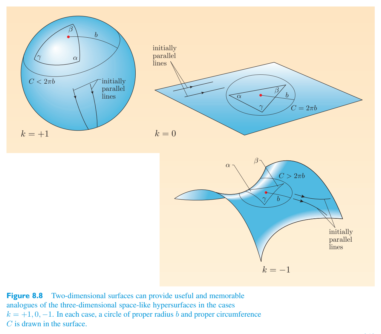
The two-dimensional spherical surface shown there is not supposed to be a picture of the three-dimensional \(k = +1\) hypersurface, but it does provide a reminder of some of the non-Euclidean features of the hypersurface. The analogy is quite far reaching. For example, on the surface of the two-dimensional sphere, triangles have interior angles that add up to more than \(\pi\) radians, and geodesics (i.e. “straight” lines) that are initially parallel will meet at some point; both of these conditions will also hold true on the \(k = +1\) space-like hypersurfaces. One other property of the spherical surface is that it has a finite total area. In a similar way, the three-dimensional space-like hypersurface has a finite total proper volume that turns out to be \(2\pi^2R^3(t)\), but like the surface of the sphere, it has no boundary, no edge, and no centre. Because of its finite volume, the kind of space described by the \(k = +1\) hypersurface is often described as closed. Sometimes the term unbounded is added to emphasize that closure does not imply an edge or any other kind of inhomogeneity. A traveller in such a space would always find it to be homogeneous and isotropic, but following a straight (i.e. geodesic) pathway would eventually bring the traveller back to points that had been visited before.图中所示的二维球面并不是三维 \(k = +1\) 超曲面的图像,但它确实提醒我们这种超曲面的一些非欧几里得特征。这个类比相当深刻。例如,在二维球面上,三角形内角和大于 \(\pi\) 弧度,最初平行的测地线(即“直线”)会在某点相交;这两个条件在 \(k = +1\) 的类空间超曲面上同样成立。球面的另一个性质是总面积有限。类似地,三维类空间超曲面具有有限的总固有体积,结果为 \(2\pi^2R^3(t)\),但像球面一样,它没有边界、没有边缘、也没有中心。由于体积有限,由 \(k = +1\) 超曲面描述的空间通常称为闭合空间。有时还会加上“无界”一词,以强调闭合并不意味着存在边缘或任何其他非均匀性。在这样的空间中,旅行者总会发现它是均匀且各向同性的;但沿直线(即测地线)前进,最终会回到曾经到过的点。
The surprising effectiveness of the spherical analogy as a source of insight into the \(k = +1\) hypersurfaces of Robertson–Walker spacetime is not really an accident. It can be shown that there is a close mathematical relationship between the points on the space-like hypersurface and the points on the three-dimensional surface of a four-dimensional sphere that might be described by the equation \(w^2+x^2+y^2+z^2=a^2\). We shall not pursue this relationship here, but embedding a space of three or more dimensions in some space of higher dimensionality is often a source of insight.球面类比能有效帮助理解罗伯逊-沃克时空的 \(k = +1\) 超曲面,这并非偶然。可以证明,类空间超曲面上的点与四维球的三维表面上的点之间存在密切的数学关系;后者可由方程 \(w^2+x^2+y^2+z^2=a^2\) 描述。我们这里不继续讨论这种关系,但把三维或更高维空间嵌入到更高维空间中,常常能带来有用的直观理解。
Case 4: \(k = -1\) and \(R^3(t)\) = constant情况 4:\(k = -1\),且 \(R^3(t)\) 为常数
Again, both spacetime and its space-like hypersurfaces will have a curved geometry. In this case, however, the proper distance grows less rapidly with the co-moving coordinate than would be the case in a flat space. In fact, as we saw earlier, \(\sigma(t)=R(t)\sinh^{-1}\chi\). A parameterized integral will again show that a circle of co-moving coordinate radius \(\chi\) has proper circumference \(2\pi R(t)\chi\), so in this case同样,时空及其类空间超曲面都具有弯曲几何。不过在这种情况下,固有距离随共动坐标增长得比平直空间中更慢。事实上,正如前面所见,\(\sigma(t)=R(t)\sinh^{-1}\chi\)。参数化积分同样会表明,共动坐标半径为 \(\chi\) 的圆具有固有周长 \(2\pi R(t)\chi\),所以在这种情况下
proper circumference of circle proper radius圆的固有周长、固有半径
Again there is an analogous surface shown in Figure 8.8, namely the saddle-shaped surface corresponding to \(k = -1\). In this case the angles of a triangle drawn around the saddle point would sum to less than \(2\pi\) radians, and there is no restriction on how big \(\chi\) can be. The \(k = -1\) hypersurface does not have a finite proper volume and is said to be open.图 8.8 还显示了一个相应的类比曲面,即对应于 \(k = -1\) 的鞍形曲面。在这种情况下,围绕鞍点画出的三角形内角和小于 \(2\pi\) 弧度,并且 \(\chi\) 可以任意大。\(k = -1\) 超曲面没有有限的固有体积,因此称为开放的。
It is interesting to note that in this case the analogy between the two-dimensional surface and the three-dimensional hypersurface is not as far reaching as it was in the \(k = +1\) case. It is simply not possible to embed a three-dimensional surface of constant negative curvature in a four-dimensional space, so the best that can be achieved is a purely local analogy.有趣的是,在这种情况下,二维表面和三维超曲面之间的类比并不像 \(k = +1\) 情况那样广泛。根本不可能将具有恒定负曲率的三维表面嵌入到四维空间中,因此可以实现的最好的结果是纯粹的局部类比。
8.3 The Friedmann equations and cosmic evolution8.3 弗里德曼方程和宇宙演化
In the previous section we introduced the Robertson–Walker metric and discussed some of its geometric features, giving particular emphasis to the meaning of the coordinates and the significance of the spatial curvature parameter k. We did this on a heuristic basis, guided by general principles such as the cosmological principle. What we did not do was to write down an energy–momentum tensor for the Universe and then look for a solution of the Einstein field equations. That is essentially what we shall do in this section. Already knowing the general form of the Robertson–Walker metric will greatly simplify this task.上一节我们介绍了罗伯逊-沃克度规并讨论了它的一些几何特征,特别强调了坐标的含义和空间曲率参数k的意义。我们在启发式的基础上做到了这一点,并遵循宇宙学原理等一般原则的指导。我们没有做的是写下宇宙的能量-动量张量,然后寻找爱因斯坦场方程的解。这本质上就是我们在本节中要做的事情。已经知道罗伯逊-沃克度规的一般形式将大大简化这项任务。
In the subsections that follow we first write down an energy–momentum tensor that is designed to represent the large-scale features of the Universe. We then substitute that energy–momentum tensor and the Robertson–Walker metric into the Einstein field equations. The result is a set of differential equations, called the Friedmann equations, that relate the Robertson–Walker parameters, k and \(R(t)\), to the densities of matter, radiation and dark energy in the Universe and to any associated pressures. Solving those equations leads us to a range of homogeneous cosmological models, each characterized by a particular form of the time-dependent scale factor \(R(t)\). In each case the scale factor encapsulates the entire expansion history of the model Universe. These models form the basis of essentially all introductions to relativistic cosmology, and are usually referred to as the Friedmann–Robertson–Walker models. It is the task of observational cosmologists to determine which, if any, of these models provides a good description of the Universe that we actually inhabit.在接下来的小节中,我们首先写下一个能量-动量张量,旨在表示宇宙的大尺度特征。然后,我们将能量-动量张量和罗伯逊沃克度规代入爱因斯坦场方程中。结果是一组微分方程,称为弗里德曼方程,它将罗伯逊-沃克参数 k 和 \(R(t)\) 与宇宙中物质、辐射和暗能量的密度以及任何相关压力联系起来。求解这些方程使我们得到一系列同质宇宙学模型,每个模型都以特定形式的时间相关尺度因子 \(R(t)\) 为特征。在每种情况下,尺度因子都封装了模型宇宙的整个膨胀历史。这些模型基本上构成了所有相对论宇宙学介绍的基础,通常被称为弗里德曼-罗伯逊-沃克模型。观测宇宙学家的任务是确定这些模型中的哪一个(如果有的话)可以很好地描述我们实际居住的宇宙。
8.3.1 The energy–momentum tensor of the cosmos8.3.1 宇宙能量-动量张量
In Chapter 4 we saw that in general relativity the sources of gravitation are contained in an energy–momentum tensor \(T_{\mu\nu}\) that describes the distribution and flow of energy and momentum in a region of spacetime. A reminder of the physical significance of the various parts of the energy–momentum tensor is given in Figure 8.9. Each of the sixteen components of \(T_{\mu\nu}\) can be measured in units of \(\mathrm{J\,m^{-3}}\) though it is often convenient to use other, equivalent, units.在第四章中,我们看到,在广义相对论中,引力源包含在能量-动量张量 \(T_{\mu\nu}\) 中,它描述了时空区域中能量和动量的分布和流动。图 8.9 提醒了能量-动量张量各个部分的物理意义。\(T_{\mu\nu}\) 的十六个分量中的每一个都可以以 \(\mathrm{J\,m^{-3}}\) 为单位进行测量,尽管使用其他等效单位通常很方便。
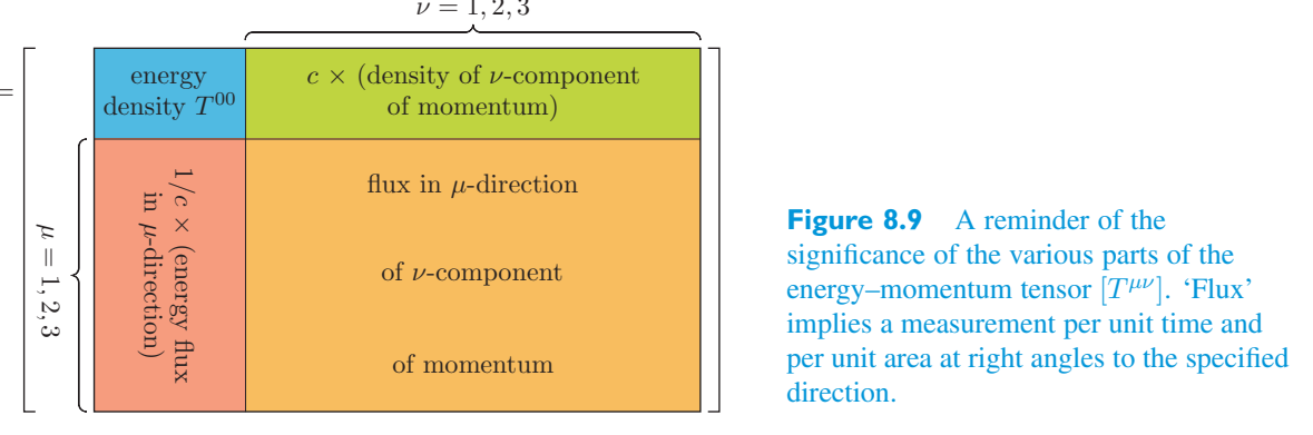
Describing in detail the distribution and flow of energy and momentum in the Universe is obviously beyond our capabilities. So, when specifying the cosmic energy–momentum tensor, cosmologists must decide on an acceptable compromise between accuracy and mathematical tractability. Traditionally, the solution is to treat the contents of spacetime as a homogeneous and isotropic ideal fluid that fills the whole of space. Such a fluid can be characterized by a proper density \(\rho(t)\) and an associated pressure \(p(t)\), each of which may depend only on the cosmic time t. According to a fundamental observer, travelling with the flow of this cosmic fluid, the fluid is locally at rest, so its energy–momentum tensor takes on the simple form that we met in Chapter 4:详细描述宇宙中能量和动量的分布和流动显然超出了我们的能力。因此,在指定宇宙能量-动量张量时,宇宙学家必须在准确性和数学易处理性之间做出可接受的折衷方案。传统上,解决方案是将时空的内容视为充满整个空间的均匀且各向同性的理想流体。这种流体的特征在于适当的密度 \(\rho(t)\) 和相关压力 \(p(t)\),其中每一个可能仅取决于宇宙时间 t。根据基本观察者的说法,随着宇宙流体的流动,流体局部处于静止状态,因此它的能量-动量张量呈现我们在第四章中遇到的简单形式:
More specifically, the current convention is to treat the contents of spacetime as a multi-component fluid composed of three distinct ideal fluids that respectively represent matter, radiation and the source of dark energy. Thus the homogeneous cosmic density can be written as更具体地说,当前的惯例是将时空的内容视为由三种不同的理想流体组成的多组分流体,这三种理想流体分别代表物质、辐射和暗能量源。因此均匀宇宙密度可以写为
and the corresponding homogeneous and isotropic cosmic pressure is相应的均匀各向同性宇宙压力为
Note that we have already taken account of the fact that the density and pressure due to dark energy are expected to be independent of time by omitting the reference to time in the case of \(\rho\) and p. It’s also worth noting that since the role of dark energy may be nothing more than emulating the effect of a cosmological constant, we shall be quite willing to consider the possibility that \(\rho\) might be negative, even though this would be ‘unphysical’ in the case of a real fluid.请注意,我们已经考虑到暗能量引起的密度和压力预计与时间无关的事实,在 \(\rho\) 和 p 的情况下省略了对时间的参考。还值得注意的是,由于暗能量的作用可能只不过是模拟宇宙学常数的影响,所以我们非常愿意考虑 \(\rho\) 可能为负的可能性,尽管这在真实流体的情况下是“非物理的”。
A few other comments about these various fluid components are in order before we move on. The first point concerns the distinction between matter and radiation. The essential difference is that particles of matter have mass, while particles of radiation (such as photons) do not. Thus, for example, protons are particles of matter but photons are particles of radiation. In the case of matter, the proper density \(\rho_{m}\) is just the usual mass density in units of \(\mathrm{kg\,m^{-3}}\), and the corresponding proper energy density is \(\rho_m c^2\). In the case of radiation, however, there is no mass density; instead, we first determine the energy density of the radiation, \(\rho_r c^2\), and then divide that by \(c^2\) to obtain an ‘effective’ mass density \(\rho_{r}\) for the radiation. It should also be noted that in some situations the mass of a certain kind of particle may be negligible, in which case the particles can be treated as radiation even though they are really particles of matter.在我们继续之前,我们还需要对这些不同的流体成分进行一些其他评论。第一点涉及物质和辐射之间的区别。本质区别在于物质粒子具有质量,而辐射粒子(例如光子)则没有质量。因此,例如,质子是物质粒子,而光子是辐射粒子。就物质而言,本征密度\(\rho_{m}\)就是通常的质量密度,单位为\(\mathrm{kg\,m^{-3}}\),相应的本征能量密度为\(\rho_m c^2\)。然而,在辐射的情况下,不存在质量密度;相反,我们首先确定辐射的能量密度 \(\rho_r c^2\),然后将其除以 \(c^2\) 以获得辐射的“有效”质量密度 \(\rho_{r}\)。还应该注意的是,在某些情况下,某种粒子的质量可能可以忽略不计,在这种情况下,即使粒子实际上是物质粒子,也可以将其视为辐射。
A second point concerns the behaviour of the density of matter and radiation as the Universe expands or contracts. Consider some large cubic region containing particles of matter and radiation. Suppose that a uniform expansion of the Universe causes each side of the cube to increase its proper length by a factor of 2 over some period of cosmic time. As a result the proper volume of the cube will increase by a factor of 8, and the proper number density of particles will decrease by a factor of 8. The expansion won’t affect the mass of each particle of matter, so the mass density of matter will also decrease by a factor of 8. In fact, there will be a general relationship between \(\rho_{m}\) and R of the form第二点涉及宇宙膨胀或收缩时物质和辐射密度的行为。考虑一些包含物质和辐射粒子的大立方区域。假设宇宙的均匀膨胀导致立方体每一面的适当长度在宇宙时间的某个时期内增加了 2 倍。这样一来,立方体的本征体积将增大 8 倍,粒子的本征数密度将减小 8 倍。膨胀不会影响每个物质粒子的质量,因此物质的质量密度也会减小 8 倍。实际上,\(\rho_{m}\) 与 R 之间存在以下形式的一般关系:
Contrast that with the behaviour of the radiation density \(\rho_{r}\), where Planck’s law (E = hf, where h is Planck’s constant) tells us that the energy E of each particle is proportional to its frequency f, and therefore inversely proportional to its wavelength \(\lambda\). That means that a doubling of R(which will also double the wavelength) halves the energy of each particle and reduces the energy density \(\rho_r c^2\) and the effective mass density \(\rho_{r}\) by a factor of 16. The general relationship for the density of radiation is therefore与辐射密度 \(\rho_{r}\) 的行为进行对比,其中普朗克定律(E = hf,其中 h 是普朗克常数)告诉我们,每个粒子的能量 E 与其频率 f 成正比,因此与其波长 \(\lambda\) 成反比。这意味着 R 加倍(也会使波长加倍)会使每个粒子的能量减半,并将能量密度 \(\rho_r c^2\) 和有效质量密度 \(\rho_{r}\) 降低 16 倍。因此,辐射密度的一般关系为
This difference in behaviour means that in an expanding Universe, the density of radiation will decline more rapidly than the density of matter, but both will decline relative to the constant density of dark energy. Figure 8.10 shows what is believed to have been the history of the various contributions to the cosmic density in our own Universe. As you can see, there may have been past epochs during which radiation and matter were each dominant, but we are now believed to inhabit a Universe that is dominated by dark energy.这种行为上的差异意味着,在膨胀的宇宙中,辐射密度的下降速度将比物质密度的下降速度更快,但两者都会相对于暗能量的恒定密度下降。图 8.10 显示了人们认为对我们宇宙中的宇宙密度的各种贡献的历史。正如你所看到的,过去可能存在辐射和物质分别占主导地位的时代,但我们现在被认为居住在一个以暗能量为主的宇宙中。
include the radiation fluid (with \(w = 1/3\)) and the dark energy fluid (with \(w = -1\)).包括辐射流体(\(w = 1/3\))和暗能量流体(\(w = -1\))。
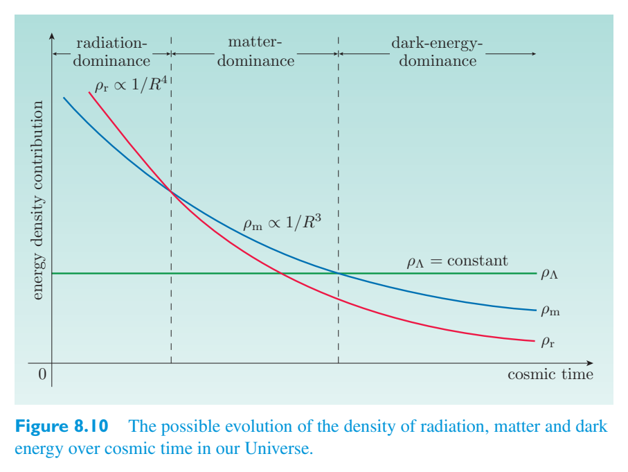
Now suppose that there is some particular time \(t_0\) (often taken to be the present time) at which \(R(t)\) has a known value \(R(t_0)\) = \(R_0\). If we use the symbols \(\rho_{m,0}\) and \(\rho_{r,0}\) to represent the values \(\rho_{m}\) (\(t_0\)) and \(\rho_{r}\) (\(t_0\)), we can write现在假设有某个特定时间 \(t_0\)(通常视为当前时间),此时 \(R(t)\) 具有已知值 \(R(t_0)\) = \(R_0\)。如果我们使用符号 \(\rho_{m,0}\) 和 \(\rho_{r,0}\) 来表示值 \(\rho_{m}\) (\(t_0\)) 和 \(\rho_{r}\) (\(t_0\)),我们可以写
So, in a model Universe where the matter is represented by pressure-free dust, there will be a uniform cosmic density因此,在物质由无压尘埃代表的宇宙模型中,将存在均匀的宇宙密度
and a corresponding homogeneous and isotropic cosmic pressure以及相应的均匀和各向同性的宇宙压力
To summarize, we have the following.总而言之,我们有以下几点。
Cosmic composition宇宙构成
At cosmic time t = \(t_0\), the sources of cosmic gravitation are specified by just three values: \(\rho_{m,0}\), \(\rho_{r,0}\) and \(\rho\). Given these three values, the cosmic density and pressure at any other cosmic time can be determined, provided that the cosmic scale factor \(R(t)\) is known as an explicit function of cosmic time.在宇宙时间 t = \(t_0\) 时,宇宙引力源仅由三个值指定:\(\rho_{m,0}\)、\(\rho_{r,0}\) 和 \(\rho\)。给定这三个值,只要宇宙尺度因子 \(R(t)\) 已知为宇宙时间的显式函数,就可以确定任何其他宇宙时间的宇宙密度和压力。
The determination of the function \(R(t)\) is the main subject of the next three subsections.函数 \(R(t)\) 的确定是接下来三小节的主要主题。
8.3.2 The Friedmann equations8.3.2 弗里德曼方程
Starting from the non-zero components of the covariant Robertson–Walker metric tensor, \(g_{00}=c^2\), \(g_{rr}=-R^2(t)/(1-kr^2)\), \(g_{\theta\theta}=-R^2(t)r^2\) and \(g_{\phi\phi}=-R^2(t)r^2\sin^2\theta\), it is time-consuming but straightforward to determine, in turn, the components of the corresponding contravariant metric tensor, the connection coefficients, the Riemann curvature components, the Ricci curvature components and the Ricci scalar (which should not be confused with the scale factor \(R\)). Once all of this has been done, the Einstein field equations can be written down using the energy–momentum tensor described in the previous subsection. Because of the many terms that vanish and the high degree of symmetry, all this calculation leads to just two independent equations, usually referred to as the Friedmann equations.从协变罗伯逊-沃克度规张量的非零分量 \(g_{00}=c^2\)、\(g_{rr}=-R^2(t)/(1-kr^2)\)、\(g_{\theta\theta}=-R^2(t)r^2\) 和 \(g_{\phi\phi}=-R^2(t)r^2\sin^2\theta\) 出发,依次求出相应的逆变度规张量分量、联络系数、黎曼曲率分量、Ricci 曲率分量和 Ricci 标量(不要把它与尺度因子 \(R\) 混淆)虽然耗时,但过程直接。完成这些之后,就可以利用上一小节描述的能量-动量张量写出爱因斯坦场方程。由于许多项为零且对称性很高,整个计算最终只给出两个独立方程,通常称为弗里德曼方程。
The Friedmann equations弗里德曼方程
The first of these equations was derived by Alexander Friedmann (Figure 8.11), a Russian mathematical physicist, in 1922, though he included a cosmological constant \(\Lambda\) that we are representing by dark energy contributions to the density \(\rho\) and pressure p. The term in square brackets on the left-hand side of the first equation is the Hubble parameter \(H(t)\) that was defined in Equation 8.17.第一个方程是由俄罗斯数学物理学家亚历山大·弗里德曼(图 8.11)于 1922 年推导出来的,尽管他包含了一个宇宙学常数 \(\Lambda\),我们用暗能量对密度 \(\rho\) 和压力 p 的贡献来表示该常数。第一个方程左侧方括号中的项是方程 8.17 中定义的哈勃参数 \(H(t)\)。
The Friedmann equations come directly from the formalism of general relativity and can be used as they stand to determine the scale factor \(R(t)\) subject to appropriate boundary conditions. However, interestingly, both equations have a very straightforward Newtonian interpretation. The first Friedmann equation is sometimes called the energy equation; it looks like a Newtonian energy equation. This impression is strengthened if the equation is rewritten as弗里德曼方程直接来自广义相对论的形式,可以直接用于确定适当边界条件下的尺度因子 \(R(t)\)。然而,有趣的是,这两个方程都有非常简单的牛顿解释。第一个弗里德曼方程有时称为能量方程;它看起来像一个牛顿能量方程。如果方程被重写为
which, apart from an overall factor representing mass, looks like a statement that the sum of the kinetic and gravitational potential energy of a particle is constant at the surface of a uniform sphere of density \(\rho\) and radius R.除了代表质量的整体因素外,它看起来像是一个陈述,即粒子的动能和引力势能之和在密度为 \(\rho\) 且半径为 R 的均匀球体表面上是恒定的。
Similarly, the second Friedmann equation is sometimes called the acceleration equation because it involves a second derivative and looks like a Newtonian equation of motion. Again, that impression is greatly strengthened if the equation is rewritten in the form同样,第二个弗里德曼方程有时也称为加速度方程,因为它涉及二阶导数并且看起来像牛顿运动方程。同样,如果将方程重写为以下形式,这种印象就会大大加强
which looks like a description of the acceleration due to (Newtonian) gravity at the surface of a sphere of radius R and uniform density \(\rho\) + \(3p/c^2\).它看起来像是对半径为 R 且密度均匀的球体表面的(牛顿)引力加速度的描述 \(\rho\) + \(3p/c^2\)。
Returning to general relativity, the Friedmann equations can still be related to energy conservation. Differentiating the energy equation and using the acceleration equation to eliminate the resulting second derivative leads to the following equation, known as the fluid equation,回到广义相对论,弗里德曼方程仍然可以与能量守恒联系起来。对能量方程求微分并使用加速度方程消除所得的二阶导数,得到以下方程,称为流体方程,
which can be shown to be an expression of energy conservation, relating changes in the energy of a co-moving volume of fluid to the work done against the external pressure.它可以被证明是能量守恒的表达式,将共动的流体能量的变化与抵抗外部压力所做的功联系起来。
The energy, acceleration and fluid equations are not all independent, but different combinations of them may be used to tackle a range of problems in cosmic evolution.能量、加速度和流体方程并不都是独立的,但它们的不同组合可以用来解决宇宙演化中的一系列问题。
Exercise 8.4 Show that the fluid equation (Equation 8.31) may be derived练习 8.4 证明可以导出流体方程(方程 8.31)
from the energy equation (Equation 8.27) and the acceleration equation (Equation 8.28).由能量方程(方程 8.27)和加速度方程(方程 8.28)得出。
Of course, when trying to solve the Friedmann equations it is necessary to make explicit the dependence on \(R(t)\) that is implicit in \(\rho(t)\) and \(p(t)\). Accepting the simplifications expressed in Equations 8.25 and 8.26, the equations that we shall use to determine the scale factor \(R(t)\) are as follows.当然,在尝试求解弗里德曼方程时,有必要明确 \(\rho(t)\) 和 \(p(t)\) 中隐含的对 \(R(t)\) 的依赖性。接受公式 8.25 和 8.26 中表示的简化,我们将使用以下公式来确定尺度因子 \(R(t)\)。
The Friedmann equations — expanded and simplified弗里德曼方程——扩展和简化
Exercise 8.5 Show that the terms in the square brackets练习8.5 证明方括号中的项
on the right of Equation 8.33 arise from the definitions of \(\rho_{m}\), \(p_{m}\), \(\rho_{r}\), \(p_{r}\), \(\rho_{\Lambda}\) and \(p_{\Lambda}\) made earlier.等式 8.33 右边的等式源自之前定义的 \(\rho_{m}\)、\(p_{m}\)、\(\rho_{r}\)、\(p_{r}\)、\(\rho_{\Lambda}\) 和 \(p_{\Lambda}\)。
8.3.3 Three cosmological models with k8.3.3 三个具有 k 的宇宙学模型
As an example of the use of the Friedmann equations, we shall briefly consider three ‘unrealistic’ single-component cosmological models. These models are chosen primarily because of their mathematical simplicity; none is thought to represent the current state of our Universe, but each still plays an important part in cosmological discussions. All three models have \(k = 0\), implying that all (fixed time) space-like hypersurfaces are geometrically flat. (As noted earlier, the flatness of three-dimensional space at fixed times does not imply that four-dimensional spacetime is geometrically flat.)作为使用弗里德曼方程的一个例子,我们将简要考虑三个“不现实”的单分量宇宙学模型。选择这些模型主要是因为它们的数学简单性;没有一个被认为代表了我们宇宙的当前状态,但每一个仍然在宇宙学讨论中发挥着重要作用。所有三个模型都有 \(k = 0\),这意味着所有(固定时间)类空间超曲面在几何上都是平坦的。 (如前所述,三维空间在固定时间的平坦度并不意味着四维时空在几何上是平坦的。)
Example 1: the de Sitter model, \(k = 0\), \(\rho\) = 0, \(\rho\)示例 1:de Sitter 模型,\(k = 0\)、\(\rho\) = 0、\(\rho\)
In this case, in addition to space being flat, there is no matter and no radiation, only dark energy. Substituting the given values into the first of the Friedmann equations, and taking the positive square root of each side, gives在这种情况下,除了空间是平坦的之外,没有物质,没有辐射,只有暗能量。将给定值代入第一个弗里德曼方程,并取每边的正平方根,得出
This is a first-order differential equation, so its solution requires one initial \(t_0\) the scale factor \(R(t_0)\) condition. We adopt the conventional choice that at t = has some known value \(R_0\). Subject to this condition, the solution can be written as这是一个一阶微分方程,因此其解需要一个初始条件 \(t_0\) 和尺度因子 \(R(t_0)\) 条件。我们采用常规选择,即在 t = 时具有某个已知值 \(R_0\)。满足这个条件,解可以写为
In this case the Hubble parameter turns out to be independent of time, since在这种情况下,哈勃参数与时间无关,因为
If we adopt - the general convention that \(H_0\) = \(H(t_0)\), then in this case we shall have \(H_0\) = 8 πGρ/3 and we can write the scale factor of this cosmological model as如果我们采用 \(H_0\) = \(H(t_0)\) 的一般约定,那么在这种情况下我们将有 \(H_0\) = 8 πGρ/3 并且我们可以将该宇宙学模型的尺度因子写为
This kind of cosmological model is known as a de Sitter model. The model was the second to be formulated and the first to describe an expanding Universe. It was proposed by Willem de Sitter in 1917, though he used a very different approach to its development and presentation. Since the model does not include any matter or radiation, it is not a good model of our current Universe but it has been used to describe a hypothetical epoch in the very early development of our Universe, known as the inflationary era, when the Universe is supposed to have undergone a brief period of very rapid expansion. It may also describe the far future of our Universe, when continued cosmic expansion will have reduced the density of matter and radiation to such an extent that those densities will be negligible compared with the (constant) density of dark energy.这种宇宙学模型被称为德西特模型。该模型是第二个被制定的模型,也是第一个描述膨胀宇宙的模型。它是由威廉·德西特 (Willem de Sitter) 于 1917 年提出的,尽管他使用了一种非常不同的方法来开发和呈现它。由于该模型不包含任何物质或辐射,因此它不是我们当前宇宙的良好模型,但它已被用来描述我们宇宙发展早期的一个假设时期,称为暴胀时代,当时宇宙被认为经历了一段非常快速膨胀的短暂时期。它还可能描述了我们宇宙的遥远未来,当时持续的宇宙膨胀将降低物质和辐射的密度,以至于与暗能量的(恒定)密度相比,这些密度可以忽略不计。
Example 2: the flat, pure radiation model, \(k = 0\), \(\rho\) = 0, \(\rho\) = 0示例 2:平坦、纯辐射模型,\(k = 0\)、\(\rho\) = 0、\(\rho\) = 0
In this case, space is flat and the Universe contains only radiation. It is thought that our Universe was almost like this during its early evolution, immediately after inflation, when it was strongly dominated by radiation. The first Friedmann equation for such a Universe gives在这种情况下,空间是平坦的,宇宙只包含辐射。人们认为,我们的宇宙在其早期演化过程中几乎就是这样,在膨胀之后,当时它受到辐射的强烈支配。这样一个宇宙的第一个弗里德曼方程给出
Adopting the usual initial condition \(R(t_0)\) = \(R_0\), the scale factor that satisfies the differential equation can again be written in terms of \(H_0\), the value of the model’s Hubble parameter at time \(t_0\). In this case采用通常的初始条件 \(R(t_0)\) = \(R_0\),满足微分方程的尺度因子可以再次写成 \(H_0\),即 \(t_0\) 时刻模型哈勃参数的值。在这种情况下
Exercise 8.6 (a) Verify that Equation 8.39 is a solution of Equation 8.38. (b) Also show that this solution implies that \(H(t)\) = 1/2 t (so H = 1/2 t), and hence confirm that it satisfies the condition \(R(t_0)\) = \(R_0\).练习 8.6 (a) 验证方程 8.39 是方程 8.38 的解。 (b) 还表明该解意味着 \(H(t)\) = 1/2 t(因此 H = 1/2 t),因此确认它满足条件 \(R(t_0)\) = \(R_0\)。
Example 3: the Einstein–de Sitter model, \(k = 0\), \(\rho\) = 0, \(\rho\) = 0示例 3:Einstein–de Sitter 模型,\(k = 0\)、\(\rho\) = 0、\(\rho\) = 0
In this case, space is flat and the Universe contains only matter. Einstein and de Sitter agreed to advocate this model in 1932, following Hubble’s discovery of cosmic expansion — hence the name Einstein–de Sitter model. Having come to disfavour the idea of a cosmological constant, they saw this model as a critical intermediate case, separating open models with \(k = -1\) from closed models with \(k = +1\). For this reason it is also often referred to as the critical model. The critical/Einstein–de Sitter model was regarded by many as providing a good description of our Universe for several decades. Its viability became increasingly suspect as observational data improved in the 1980s, but it wasn’t until the late-1990s that it was finally abandoned in favour of models dominated by dark matter.在这种情况下,空间是平坦的,宇宙只包含物质。在哈勃发现宇宙膨胀之后,爱因斯坦和德西特于 1932 年同意提倡这个模型,因此得名爱因斯坦-德西特模型。由于不赞成宇宙学常数的概念,他们将此模型视为关键的中间情况,将 \(k = -1\) 的开放模型与 \(k = +1\) 的封闭模型分开。因此,它通常也被称为临界模型。几十年来,批判/爱因斯坦-德西特模型被许多人认为提供了对我们宇宙的良好描述。随着 20 世纪 80 年代观测数据的改善,它的可行性变得越来越令人怀疑,但直到 90 年代末,它最终被放弃,取而代之的是以暗物质为主的模型。
The first Friedmann equation for an Einstein–de Sitter Universe can be written as爱因斯坦-德西特宇宙的第一个弗里德曼方程可以写为
With \(R(t_0)\) = \(R_0\), the solution can be written as对于 \(R(t_0)\) = \(R_0\),解可以写为
In this case the Hubble parameter is given by \(H(t)\) = 2在这种情况下,哈勃参数由 \(H(t)\) = 2 给出
The variation of R with t for all three of the models that we have been discussing is shown in Figure 8.12. Diagrams of this kind provide a useful way of visualizing the expansion history of a cosmological model. You will see more such diagrams in the next section.我们讨论的所有三个模型的 R 随 t 的变化如图 8.12 所示。此类图表提供了一种可视化宇宙学模型的膨胀历史的有用方法。您将在下一节中看到更多此类图表。
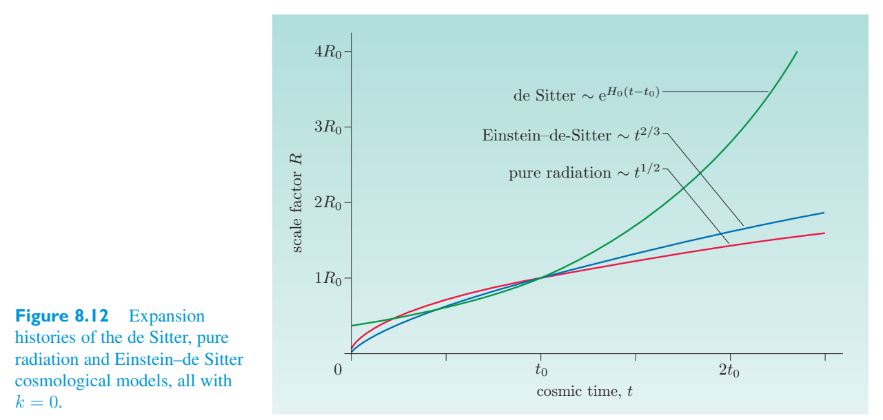
In a Universe where \(k = 0\), it follows from the first Friedmann equation and the definition of the Hubble parameter (\(H(t)\) = R − 1 d R/d在 \(k = 0\) 的宇宙中,根据第一个弗里德曼方程和哈勃参数的定义 (\(H(t)\) = R − 1 d R/d
So, as a \(k = 0\) Universe expands or contracts, the cosmic density must change for a \(k = 0\) in proportion to the square of the Hubble parameter. Moreover, Universe, the changing value of the total cosmic density will always have the value implied by Equation 8.42; this value is called the critical density. It is denoted by \(\rho\) c (t) and is given by the following.因此,当 \(k = 0\) 宇宙膨胀或收缩时,\(k = 0\) 的宇宙密度必须与哈勃参数的平方成比例地变化。而且,宇宙,总宇宙密度的变化值将始终具有方程8.42所暗示的值;该值称为临界密度。它被表示为\(\rho\) c (t)并且由以下给出。
Critical density临界密度
The critical density provides a useful reference density that we shall make use of in the next subsection. The key points of the three flat space models considered in this subsection are summarized in Table 8.1.临界密度提供了一个有用的参考密度,我们将在下一小节中使用它。表 8.1 总结了本小节中考虑的三个平坦空间模型的要点。
Table 8.1 Spatially flat (\(k = 0\)) single-component models.表 8.1 空间平坦 (\(k = 0\)) 单组件模型。
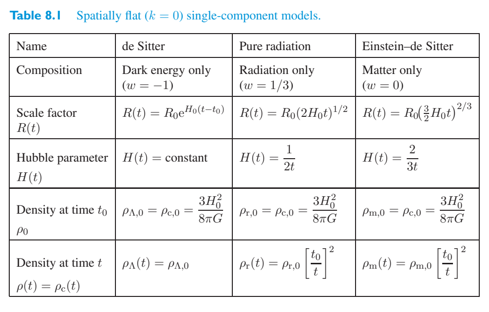
Name de Sitter Pure radiation Einstein–de Sitter德西特纯辐射爱因斯坦-德西特
Composition Dark energy only Radiation only Matter only (\(w = -1\)) (\(w = 1/3\)) (\(w = 0\))成分仅暗能量仅辐射仅物质 (\(w = -1\)) (\(w = 1/3\)) (\(w = 0\))
Scale factor尺度因子
Hubble parameter \(H(t)\) = co nstant哈勃参数 \(H(t)\) = 常数
Density at time t \(\rho\) = \(\rho\) =时间 t 处的密度 \(\rho\) = \(\rho\) =
Density at time t \(\rho(t)\) = \(\rho\)时间 t 处的密度 \(\rho(t)\) = \(\rho\)
8.3.4 Friedmann–Robertson–Walker models in general8.3.4 弗里德曼-罗伯逊-沃克模型概述
A relativistic cosmological model based on the Robertson–Walker metric with a scale factor determined by the Friedmann equations is known as a Friedmann–Robertson–Walker (FRW) model. The three single-component models with \(\rho\) = \(\rho\) c and hence \(k = 0\) that we considered in the previous subsection are among the simplest examples of FRW models. When specifying a general FRW model it is conventional to express each of the densities as a fraction of the critical density \(\rho\) c. These fractional densities are called density parameters and are defined as follows.基于罗伯逊-沃克度规的相对论宇宙学模型,其尺度因子由弗里德曼方程确定,称为弗里德曼-罗伯逊-沃克(FRW)模型。 \(\rho\) = \(\rho\) c 的三个单分量模型以及我们在上一小节中考虑的 \(k = 0\) 是 FRW 模型最简单的示例。当指定通用 FRW 模型时,通常将每个密度表示为临界密度 \(\rho\) c 的分数。这些分数密度称为密度参数,定义如下。
Density parameters密度参数
Note that although the density \(\rho\) is independent of time, the density parameter \(\Omega\) is not; this is because of the time dependence of \(\rho\) c.请注意,虽然密度 \(\rho\) 与时间无关,但密度参数 \(\Omega\) 却不然;这是因为 \(\rho\) 的时间依赖性 c.
Using the density parameters, the first Friedmann equation can be rewritten as使用密度参数,第一个弗里德曼方程可以重写为
Rearranging this to read重新排列此内容以阅读
it can be seen that at any time the total density parameter determines the cosmic geometry of space, since可以看出,在任何时刻,总密度参数决定了空间的宇宙几何形状,因为
When it comes to solving the Friedmann equations, a few special cases, such as those considered in the previous subsection, can be treated analytically. However, it is often necessary to resort to numerical methods to find solutions. Some illustrative examples of the kinds of solutions that arise are shown in Figure 8.13.在求解弗里德曼方程时,可以分析地处理一些特殊情况,例如上一小节中考虑的情况。然而,通常需要借助数值方法来寻找解决方案。图 8.13 显示了所出现的解决方案类型的一些说明性示例。
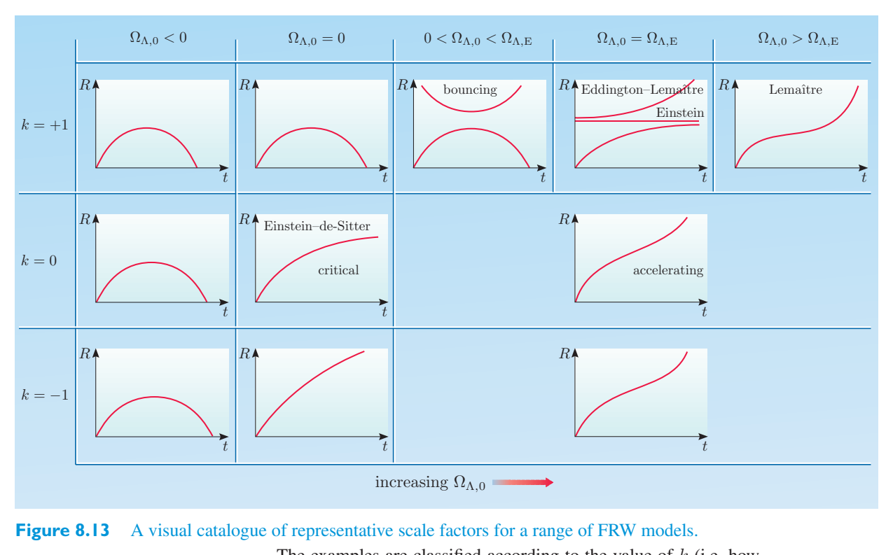
The examples are classified according to the value of k (i.e. how \(\Omega_{m,0}\) + \(\Omega_{r,0}\) + \(\Omega_{\Lambda,0}\) compares with 1) and the value of \(\Omega_{\Lambda,0}\). In most cases the small graph of R against t that appears in any given cell is intended to be representative of the whole class of specific results that would emerge for different choices of \(\Omega_{m,0}\), \(\Omega_{r,0}\) and \(\Omega_{\Lambda,0}\). Of course, this means that some important cases are not properly illustrated. For instance, the exponentially expanding de Sitter model sits in the cell devoted to \(k = 0\) and \(\Omega_{\Lambda,0}\) > 0, but the graph that appears in that cell is for a model that contains some matter and radiation, which the de Sitter model does not. You can imagine the de Sitter model as a limiting case of the model that is shown.这些示例根据 k 的值(即 \(\Omega_{m,0}\) + \(\Omega_{r,0}\) + \(\Omega_{\Lambda,0}\) 与 1 进行比较)和 \(\Omega_{\Lambda,0}\) 的值进行分类。在大多数情况下,出现在任何给定单元格中的 R 与 t 的小图旨在代表针对 \(\Omega_{m,0}\)、\(\Omega_{r,0}\) 和 \(\Omega_{\Lambda,0}\) 的不同选择而出现的整类特定结果。当然,这意味着一些重要的案例没有得到适当的说明。例如,呈指数扩展的德西特模型位于专用于 \(k = 0\) 和 \(\Omega_{\Lambda,0}\) > 0 的单元中,但该单元中出现的图形适用于包含某些物质和辐射的模型,而德西特模型则不包含这些物质和辐射。您可以将 de Sitter 模型想象为所示模型的极限情况。
In fact, the general kind of model shown in the \(k = 0\), \(\Omega_{\Lambda,0}\) > 0 cell is of special interest to cosmologists. It is currently thought to provide a good description of the large-scale features of our Universe. Like many of the models, it starts with \(R=0\) and growing. This is an indication of an early phase in cosmic evolution that would have been dense and hot. It corresponds to the statement that the Universe began with a Big Bang. The high density is a simple consequence of the smallness of R at early times; we have already seen that \(\rho_{m}\) ∝ 1/\(R^3\), while for the radiation that dominated the early Universe, \(\rho_{m}\) ∝ 1/\(R^4\). The high temperature, T, follows from the 1/\(R^4\) dependence of the energy density and the expectation that the radiation was thermal radiation, implying (in accordance with Stefan’s law) that its energy density is proportional to \(T^{4}\) with the consequence that T ∝ 1/R. Thus the temperature would also have been higher in the compressed conditions of the early Universe.事实上,宇宙学家对 \(k = 0\)、\(\Omega_{\Lambda,0}\) > 0 单元中显示的一般模型特别感兴趣。目前认为它可以很好地描述我们宇宙的大尺度特征。与许多模型一样,它以 \(R=0\) 开头并不断增长。这表明宇宙演化的早期阶段是稠密且炎热的。它对应于宇宙始于大爆炸的说法。高密度是早期 R 较小的简单结果;我们已经看到 \(\rho_{m}\) ∝ 1/\(R^3\),而对于主导早期宇宙的辐射,\(\rho_{m}\) ∝ 1/\(R^4\)。高温 T 是根据能量密度的 1/\(R^4\) 依赖性以及辐射为热辐射的预期得出的,这意味着(根据斯特凡定律)其能量密度与 \(T^{4}\) 成正比,因此 T ∝ 1/R。因此,在早期宇宙的压缩条件下,温度也会更高。
Another interesting feature of this kind of model is that although it indicates continuous expansion (R always gets bigger), it also shows that the rate of expansion initially declines but then begins to increase again. For that reason this is sometimes described as an accelerating model. The acceleration in the rate of expansion is a result of the changing densities of matter, radiation and dark energy. The model is characterized by \(k = 0\), so the sum of those densities will always be the critical density \(\rho\) c, but as the critical density itself declines, the proportions contributed by matter, radiation and dark energy will change, with dark energy eventually becoming dominant. (Look again at Figure 8.10.) During the eras when radiation and matter are dominant, the rate of expansion decelerates, but when dark matter becomes dominant, the rate of expansion accelerates. We shall have more to say about this model in the next section.这种模型的另一个有趣的特点是,虽然它表明持续扩张(R总是变大),但它也表明扩张率最初下降,但随后又开始增加。因此,这有时被描述为加速模型。膨胀率的加速是物质、辐射和暗能量密度变化的结果。该模型的特征为 \(k = 0\),因此这些密度的总和将始终为临界密度 \(\rho\) c,但随着临界密度本身的下降,物质、辐射和暗能量所贡献的比例将发生变化,最终暗能量占据主导地位。(再看看图8.10。)在辐射和物质占主导地位的时代,膨胀速度会减慢,但当暗物质占主导地位时,膨胀速度会加快。我们将在下一节中更多地讨论这个模型。
Looking more generally at the FRW models in Figure 8.13, you can see that if \(\Omega_{\Lambda,0}\) < 0, as in the column on the left, the model generally starts with a Big Bang but eventually reaches a state of maximum expansion and then recollapses. Its end would involve a state of increasing density as R decreases to zero in a process usually referred to as the big crunch. These recollapsing models occur with all possible values of k, so their space-like hypersurfaces may be open, flat or closed, depending on which particular variant we choose to study.更一般地看一下图 8.13 中的 FRW 模型,您可以看到,如果 \(\Omega_{\Lambda,0}\) < 0,如左侧的列所示,模型通常以大爆炸开始,但最终达到最大膨胀状态,然后重新塌陷。它的最终结果将是随着 R 减小到零,密度不断增加的状态,这个过程通常被称为“大紧缩”。这些塌陷模型以所有可能的 k 值出现,因此它们的类空间超曲面可能是开放的、平坦的或封闭的,具体取决于我们选择研究的特定变体。
The \(\Omega_{\Lambda,0}\) = 0 models in the middle column include open, ever-expanding models, closed, recollapsing models and, in between, the flat space \(k = 0\) models that will include the Einstein–de Sitter model and the flat, pure radiation model.中间一列的 \(\Omega_{\Lambda,0}\) = 0 模型包括开放的、不断膨胀的模型、封闭的、塌陷的模型,以及介于两者之间的平坦空间 \(k = 0\) 模型,其中包括爱因斯坦-德西特模型和平坦的纯辐射模型。
The set of \(\Omega_{\Lambda,0}\) > 0 models includes the \(k = 0\) accelerating model that we have already discussed, a similar \(k = -1\) open model, and several different closed models, including some that do not feature a Big Bang. A particularly interesting case amongst this latter class is the static Einstein model, represented by a horizontal R against t graph. This, you will recall, was the first relativistic cosmological model, the one that prompted Einstein to introduce the cosmological constant. Ignoring the effect of radiation (i.e. setting \(\Omega_{r,0}\) = 0), the Einstein model arises when the effect of dark energy exactly balances the effect of matter to ensure that d R/d t = \(d^2 R\)/\((dt)^2\) = 0, so that R has the constant value R. For this to be the case, it follows from the second Friedmann equation (Equation 8.33) that \(\rho\) = \(\rho_{m,0}\)/2, or, in terms of density parameters,\(\Omega_{\Lambda,0}\) > 0 模型集包括我们已经讨论过的 \(k = 0\) 加速模型、类似的 \(k = -1\) 开放模型和几个不同的封闭模型,包括一些不具有大爆炸特征的模型。后一类中一个特别有趣的例子是静态爱因斯坦模型,由水平 R 与 t 图表示。您可能还记得,这是第一个相对论宇宙学模型,促使爱因斯坦引入宇宙学常数。忽略辐射的影响(即设置 \(\Omega_{r,0}\) = 0),当暗能量的影响恰好平衡物质的影响,确保 d R/d t = \(d^2 R\)/\((dt)^2\) = 0 时,爱因斯坦模型就产生了,从而使 R 具有恒定值 R。对于这种情况,根据第二个弗里德曼方程(方程 8.33)得出 \(\rho\) = \(\rho_{m,0}\)/2,或者,就密度参数而言,
This is the value of the dark energy density parameter that is indicated by \(\Omega_E\) in Figure 8.13.这是暗能量密度参数的值,如图 8.13 中的 \(\Omega_E\) 所示。
One other model that deserves to be mentioned is the Eddington–Lemaître model (\(k = +1\), \(\Omega_{\Lambda,0}\) = \(\Omega_E\)). This was brought to prominence in a 1927 report on expanding-universe models by Georges Lemaître (1894–1966), a Belgian catholic priest and cosmologist. The model was strongly supported by Sir Arthur Eddington – hence the name. It is unusual in that it does not start with a big bang. Rather it can develop from the (static) Einstein model, which is actually unstable against fluctuations in the density. In 1933 Lemaître proposed a primitive variant of Big Bang theory as an explanation of the origin of the Universe, and shifted his (\(k = +1\), \(\Omega_{\Lambda,0}\) > \(\Omega_E\)). allegiance to the model now known as the Lemaître model另一个值得一提的模型是 Eddington–Lemaître 模型 (\(k = +1\), \(\Omega_{\Lambda,0}\) = \(\Omega_E\))。比利时天主教神父兼宇宙学家 Georges Lemaître(1894-1966 年)在 1927 年发表的关于膨胀宇宙模型的报告中,这一点得到了突出强调。该模型得到了阿瑟·爱丁顿爵士的大力支持——因此得名。它的不同寻常之处在于它并不是从大爆炸开始的。相反,它可以从(静态)爱因斯坦模型发展而来,该模型实际上对密度波动不稳定。 1933年,Lemaître提出了大爆炸理论的原始变体作为宇宙起源的解释,并改变了他的理论(\(k = +1\),\(\Omega_{\Lambda,0}\) > \(\Omega_E\))。效忠现在称为 Lemaître 模型的模型
Exercise 8.7 Using the first Friedmann equation, show练习8.7 使用第一个弗里德曼方程,显示
that in Einstein’s static Universe R = (\(c^2\)/4 πGρ) 1/2, and evaluate this in light-years and parsecs given that a modern estimate of the current cosmic matter density is \(\rho\) ≈ \(3\times10^{-27}\) kg.在爱因斯坦的静态宇宙中,R = (\(c^2\)/4 πGρ) 1/2,并以光年和秒差距来评估这一点,因为当前宇宙物质密度的现代估计是 \(\rho\) ≈ \(3\times10^{-27}\) kg。
Exercise 8.8 Using the second Friedmann equation,练习8.8 使用第二个弗里德曼方程,
show that if \(\Omega_{r,0}\) is taken to be zero, the condition that distinguishes those FRW Universes that have already started to (positively) accelerate at time \(t_0\) from those that have not is \(\Omega\) ≥ \(\Omega\)/2.表明,如果 \(\Omega_{r,0}\) 取为零,则区分那些在 \(t_0\) 时间已经开始(正)加速的 FRW 宇宙与那些尚未开始加速的 FRW 宇宙的条件是 \(\Omega\) ≥ \(\Omega\)/2。
Exercise 8.9 Assuming that \(\Omega_{r,0}\) is negligible, the练习 8.9 假设 \(\Omega_{r,0}\) 可以忽略不计,则
range of FRW models can be represented by points in a plane with coordinates \(\Omega_{m,0}\) and \(\Omega_{\Lambda,0}\), as indicated in Figure 8.14. Write down the condition that determines the location models with \(k = -1\), of the dividing line between models with \(k = +1\) and and identify the point or points associated with (i) the de Sitter model, (ii) the Einstein–de Sitter model, and (iii) the Einstein model.FRW 模型的范围可以用坐标为 \(\Omega_{m,0}\) 和 \(\Omega_{\Lambda,0}\) 的平面上的点来表示,如图 8.14 所示。写下确定 \(k = -1\) 位置模型的条件,以及 \(k = +1\) 模型之间分界线的条件,并识别与 (i) 德西特模型、(ii) 爱因斯坦-德西特模型和 (iii) 爱因斯坦模型相关的一个或多个点。
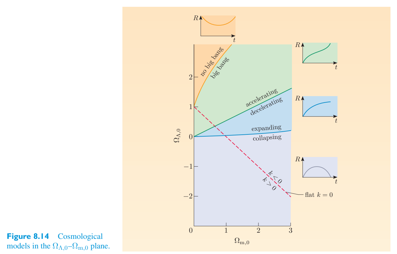
8.4 Friedmann–Robertson–Walker models and observations8.4 弗里德曼-罗伯逊-沃克模型和观察
In this section we consider the relationship between certain observable properties of the Universe in which we live, and the parameters that have played an important part in our discussion of cosmological models, particularly the proper distance (\(\sigma\) or d p), the Hubble parameter \(H(t)\) and the cosmic time t. We said earlier that \(t_0\) is often taken to represent the current cosmic time. From this point on, that will always be the case.在本节中,我们考虑我们所生活的宇宙的某些可观测特性与在我们讨论宇宙学模型中发挥重要作用的参数之间的关系,特别是固有距离(\(\sigma\)或d p)、哈勃参数\(H(t)\)和宇宙时间t。我们之前说过\(t_0\)经常被用来代表当前的宇宙时间。从现在开始,情况将永远如此。
8.4.1 Cosmological redshift and cosmic expansion8.4.1 宇宙学红移和宇宙膨胀
Defining redshift定义红移
The redshift of spectral lines is a common and useful phenomenon in astronomy. In earlier chapters we have encountered two distinct causes of redshift.谱线红移是天文学中常见且有用的现象。在前面的章节中,我们遇到了红移的两个不同原因。
1. The Doppler effect of special relativity, which arises when a source of1. 狭义相对论的多普勒效应,当源
radiation and the observer of that radiation are in relative motion.辐射和该辐射的观察者处于相对运动。
2. The gravitational redshift of general relativity that is a consequence of the2. 广义相对论的引力红移是
gravitational time dilation that exists between observers who are relatively at rest but located in regions of different spacetime curvature.相对静止但位于不同时空曲率区域的观察者之间存在的引力时间膨胀。
You are about to encounter a third cause of redshift, usually referred to as cosmological redshift, that arises when the source and the observer are separated by cosmologically large distances in a Universe that is contracting or expanding.您将遇到红移的第三个原因,通常称为宇宙学红移,当源和观察者在收缩或膨胀的宇宙中相距很远的宇宙学距离时,就会出现红移。
For our present purposes it is useful to introduce a quantitative measure of the redshift of a spectral line. This quantity is widely used in astronomy and is defined as follows.就我们目前的目的而言,引入光谱线红移的定量测量是有用的。该量在天文学中广泛使用,定义如下。
Quantitative definition of redshift红移的定量定义
Here \(\lambda\) em is the wavelength at which some spectral line is emitted, as measured at the source (or, more realistically, as determined from some laboratory-based experiment involving similar sources), and \(\lambda\) ob is the observed wavelength of the spectral line when it reaches its distant observer. Note that z is a dimensionless ratio, so it’s just represented by a number such as 0.1 or 2. A negative value of z is used to indicate a blueshift. In most cases of astronomical interest, all the lines in a spectrum will have the same redshift, so the measured redshift is a property of the body concerned, not just the spectral line.这里 \(\lambda\) em 是在光源处测量的某些谱线发射的波长(或者更实际地,根据涉及类似源的一些基于实验室的实验确定),而 \(\lambda\) ob 是当光谱线到达其远处观察者时观察到的波长。请注意,z 是无量纲比率,因此仅用 0.1 或 2 等数字表示。z 的负值用于表示蓝移。在大多数天文兴趣的情况下,光谱中的所有谱线都将具有相同的红移,因此测量到的红移是相关天体的属性,而不仅仅是谱线的属性。
- ● Show that when expressed in terms of the emitted and observed frequencies,证明当用发射频率和观测频率表示时,
\(f_{\rm em}\) and f ob, the definition of redshift implies that\(f_{\rm em}\) 和 f ob,红移的定义意味着
f \(\lambda\), ❍ From Equation 8.51 using the general relation c =f \(\lambda\), ❍ 根据公式 8.51,使用一般关系 c =
Adding 1 to each side gives the required result, which we shall use later.每边加 1 就得到了我们稍后将使用的所需结果。
Relating redshift to the scale factor将红移与尺度因子相关
Suppose that a fundamental observer, at the origin of co-moving coordinates in a Robertson–Walker spacetime, observes a light signal emitted from a distant galaxy at a fixed radial co-moving coordinate r = \(\chi\). We can take the coordinates of the emission event to be (t em, \(\chi\), 0, 0) and the coordinates of the observation event to be (t ob, 0, 0, 0). The light signal will travel along a null geodesic where (d s) 2 = 0, so it follows from the Robertson–Walker line element that all along that null geodesic,假设一个基本观察者在罗伯逊-沃克时空中的共动坐标原点处观察到从遥远星系在固定径向共动坐标 r = \(\chi\) 处发出的光信号。我们可以将发射事件的坐标设为(t em, \(\chi\), 0, 0),将观测事件的坐标设为(t ob, 0, 0, 0)。光信号将沿着零测地线传播,其中 (d s) 2 = 0,因此从罗伯逊-沃克线元可以得出,沿着该零测地线,
Splitting this expression into time-dependant and space-dependant parts, and taking the positive square root, we get将该表达式分解为时间相关部分和空间相关部分,并取正平方根,我们得到
Integrating each part over the whole pathway,整合整个路径的每个部分,
Now suppose that a second signal is emitted from the same source a short time later, at t em + δt em, and that it is observed a short time after the first signal, at t ob + δt ob. This second signal also travels along a null geodesic, so现在假设在 t em + δt em 处不久后从同一源发出第二个信号,并且在第一个信号后不久(在 t ob + δt ob 处)观察到第二个信号。第二个信号也沿着零测地线传播,因此
The spatial integral is the same in both cases since it only involves co-moving coordinates. Consequently we can equate the two time-dependent integrals:两种情况下的空间积分是相同的,因为它只涉及共动的坐标。因此,我们可以将两个与时间相关的积分等同:
Now, each of these integrals can be written as the sum of two parts. For the integral on the left,现在,这些积分中的每一个都可以写成两部分的和。对于左边的积分,
and for the integral on the right,对于右边的积分,
Subtracting the corresponding sides of these two equations, we see that减去这两个方程的对应边,我们可以看到
Rearranging and cancelling the factor c, we see that重新排列并取消因子 c,我们看到
but each of these integrals covers a very short period of time, so the integrand will be effectively constant for the short duration of the integration, and we can write但每个积分都涵盖很短的时间,因此被积函数在积分的短时间内实际上是恒定的,我们可以写
It follows that由此可见
If we now let δt em be the proper period of oscillation of the emitted light, then δt ob will be the period of the observed light and we can use the fact that frequency is inversely proportional to period to replace δt em/δt ob by f ob/\(f_{\rm em}\), giving如果我们现在让 δt em 为发射光的固有振荡周期,则 δt ob 将是观测到的光的周期,我们可以利用频率与周期成反比的事实,用 f ob/\(f_{\rm em}\) 代替 δt em/δt ob,得到
Substituting this result into Equation 8.52, we obtain our final result.将此结果代入公式 8.52,我们得到最终结果。
Cosmological redshift related to scale factor与尺度因子相关的宇宙红移
So the redshift of the light is determined by the ratio of the scale factors at the times of observation and emission. In an expanding Universe, R(t ob) will be bigger than R(t em), so Equation 8.56 predicts that the observed light will be positively redshifted. If the Universe expands monotonically, then the more distant the source of the light, the longer the time the light will spend in transit, and, generally speaking, the greater will be the observed redshift.因此,光的红移是由观察时和发射时的尺度因子之比决定的。在膨胀的宇宙中,R(t ob) 将大于 R(t em),因此方程 8.56 预测观测到的光将发生正红移。如果宇宙单调膨胀,那么光源越远,光传输的时间就越长,一般来说,观察到的红移就越大。
- ● A distant quasar has a redshift z = 6.0. By what factor has the Universe遥远的类星体的红移 z = 6.0。宇宙是由什么因素构成的
expanded since the quasar emitted the light that we receive today? ❍ Substituting z = 6.0 in Equation 8.56 gives \(R(t)\)/\(R(t)\) = 7.自从类星体发出我们今天收到的光以来就膨胀了? ❍ 将 z = 6.0 代入公式 8.56,得出 \(R(t)\)/\(R(t)\) = 7。
Note that although galaxies participating in the Hubble flow will have a proper radial velocity away from any fundamental observer, any cosmological redshift that such observers measure is not a Doppler effect. The formula for cosmological redshift is quite different from the Doppler formula. However, what might be described as the effect of ‘cosmological motion’ (i.e. the Hubble flow, not the peculiar motions of individual galaxies or non-fundamental observers) is automatically included in the calculation of cosmological redshift, so there is no need for any kind of additional ‘Doppler correction’ to account for that motion. A common way of expressing this is to say that cosmological redshift is a result of motion that arises from the expansion of space rather than motion through space. Figure 8.15 overleaf illustrates this view. It indicates a cosmological redshift that is a consequence of the expansion of space and the corresponding stretching of wavelength while the radiation is in transit between galaxies with fixed co-moving coordinates. The galaxies themselves are supposed to be bound systems, so they are not enlarged by the stretching of space, which can be thought of as a weak ‘background’ effect that becomes significant only on the cosmic scale.请注意,尽管参与哈勃流的星系将具有远离任何基本观察者的适当径向速度,但此类观察者测量到的任何宇宙红移都不是多普勒效应。宇宙学红移公式与多普勒公式有很大不同。然而,可以被描述为“宇宙运动”的影响(即哈勃流,而不是单个星系或非基本观察者的特殊运动)会自动包含在宇宙红移的计算中,因此不需要任何额外的“多普勒校正”来解释该运动。表达这一点的一种常见方式是,宇宙学红移是空间膨胀引起的运动的结果,而不是空间运动的结果。背面图 8.15 说明了这一视图。它表明宇宙学红移是当辐射在具有固定共动坐标的星系之间传输时空间膨胀和相应的波长拉伸的结果。星系本身被认为是束缚系统,因此它们不会因空间的拉伸而扩大,这可以被认为是一种弱的“背景”效应,只有在宇宙尺度上才会变得重要。
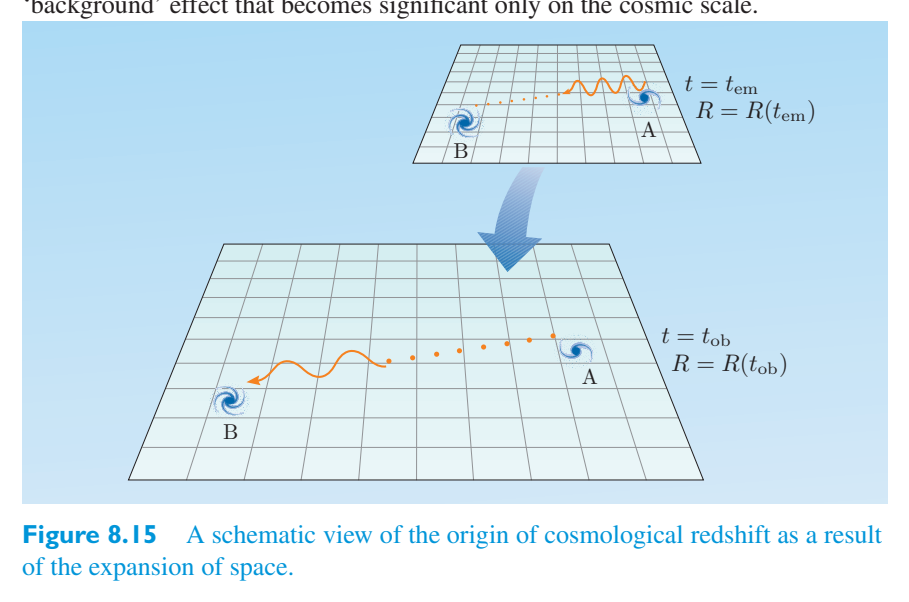
Exercise 8.10 Can we reasonably expect to measure练习 8.10 我们能否合理预期测量
a change in the value of \(R(t)\) by means of local experiments, such as the observation of cosmological redshifts in the spectra of nearby stars?通过局部实验(例如观察附近恒星光谱中的宇宙红移)来改变 \(R(t)\) 的值?
Relating redshift to a measurable distance将红移与可测量的距离联系起来
The relation between redshift and the scale factor is an important step towards linking the cosmological models that we have been developing with observations, but the scale factor itself is not directly measurable. To obtain a relationship that we can test, we still need to relate the redshift to some other quantity that astronomers can actually measure. The most suitable quantity is the luminosity distance, d L. This is defined in terms of the luminosity L of an isotropically radiating source and the energy flux F that reaches the observer, so that红移和尺度因子之间的关系是将我们一直在开发的宇宙学模型与观测联系起来的重要一步,但尺度因子本身是不可直接测量的。为了获得我们可以测试的关系,我们仍然需要将红移与天文学家可以实际测量的其他一些量联系起来。最合适的量是光度距离 d L。这是根据各向同性辐射源的光度 L 和到达观察者的能量通量 F 来定义的,因此
Here 4 πd 2 L represents the area over which the radiation emitted in unit time is spread when it reaches the observer.这里 4 πd 2 L 表示单位时间内发出的辐射到达观察者时所扩散的面积。
In a static Euclidean space d L would be equal to the coordinate distance of the source. However, in Robertson–Walker spacetime things are not so simple. Consider a fundamental observer making observations from the origin. For a source at radial co-moving coordinate r = \(\chi\), the proper area of the sphere over which the radiation is spread when it reaches the observer at time t ob can be shown to be 4 πR 2 (t ob) \((\chi)^2\). However, we saw earlier, in Equation 8.54, that in an expanding Universe, radiation emitted over a time period δt em will be observed over a longer time period δt ob, so the observed energy flux will be reduced by a factor在静态欧几里得空间中,d L 将等于源的坐标距离。然而,在罗伯逊-沃克时空中,事情就没那么简单了。考虑一个基本观察者从原点进行观察。对于径向共动坐标 r = \(\chi\) 处的源,当辐射在时间 t ob 到达观察者时,辐射在其上传播的球体的适当面积可以显示为 4 πR 2 (t ob) \((\chi)^2\)。然而,我们之前在方程 8.54 中看到,在膨胀的宇宙中,在一段时间 δt em 内发射的辐射将在更长的时间段 δt ob 内观测到,因此观测到的能量通量将减少一个因子
We have also seen that in an expanding Universe, the wavelength of each arriving photon will be stretched out, so its energy will be reduced and the observed energy flux will therefore be further reduced by a factor我们还看到,在膨胀的宇宙中,每个到达光子的波长将被拉长,因此其能量将减少,观测到的能量通量将进一步减少一个因子
Consequently, in an FRW Universe at time t ob,因此,在时间 t ob 的 FRW 宇宙中,
Comparing Equations 8.57 and 8.60, it can be seen that比较式 8.57 和 8.60 可以看出
To obtain a relation between luminosity distance and redshift, we now need to express the quantity R(t ob) \(\chi\) in terms of z. This is actually quite tricky, though the method and result are both well known. There is an exact method valid for all values of z and an approximate method valid for z(1. Let’s deal with the approximate method first; we shall come back to the exact method in the next subsection. The first step is to use Taylor’s theorem to expand the scale factor \(R(t)\) at some general time t as a power series in the lookback time, (\(t_0\) − t), about its current value \(R(t_0)\). This series can be written as为了获得光度距离和红移之间的关系,我们现在需要用 z 来表达 R(t ob) \(\chi\) 量。这实际上是相当棘手的,尽管方法和结果都是众所周知的。有一个对所有 z 值都有效的精确方法和一个对 z(1 有效的近似方法。让我们首先处理近似方法;我们将在下一小节中回到精确方法。第一步是使用泰勒定理将尺度因子 \(R(t)\) 在某个一般时间 t 展开为回溯时间 (\(t_0\) − t) 中的幂级数,关于其当前值 \(R(t_0)\)。这个系列可以写成
where \(H_0\) is the current value of the Hubble parameter \(H(t)\) that was introduced in Equation 8.17,其中 \(H_0\) 是公式 8.17 中引入的哈勃参数 \(H(t)\) 的当前值,
and q 0 is the current value of the deceleration parameter q (t) defined byq 0 是由下式定义的减速度参数 q (t) 的当前值
This series is used in conjunction with Equation 8.53 (which involves the co-moving coordinate \(\chi\) and the scale parameter \(R(t)\)) and the relation that we have already found that relates the scale parameter to the redshift, 1 + z = \(R(t)\)/\(R(t)\). The result, after some labour, is that for observations该级数与方程 8.53(涉及共动坐标 \(\chi\) 和尺度参数 \(R(t)\))以及我们已经发现的尺度参数与红移的关系 1 + z = \(R(t)\)/\(R(t)\) 结合使用。经过一番努力后,结果是用于观察
Remembering that this is valid only for small values of z, the relationship tells us that, to a first approximation, and ignoring any peculiar motion, we should expect to find that the redshift of each galaxy is proportional to its luminosity distance.请记住,这仅适用于较小的 z 值,该关系告诉我们,对于第一个近似值,并忽略任何特殊运动,我们应该期望发现每个星系的红移与其光度距离成正比。
Here the constant of proportionality \(H_0\) is the current value of the Hubble parameter. In addition, if we make more precise observations, particularly if they involve somewhat larger redshifts (though still significantly less than 1), then we should expect to see deviations from the simple proportional behaviour, and these should, in principle at least, inform us about any acceleration or deceleration of the cosmic expansion via q 0. A graph of the relationship between d L and z, for a range of values of q 0 and a realistic value of \(H_0\), is shown in Figure 8.16.这里比例常数 \(H_0\) 是哈勃参数的当前值。此外,如果我们进行更精确的观测,特别是如果它们涉及更大的红移(尽管仍然明显小于 1),那么我们应该期望看到与简单比例行为的偏差,并且这些应该至少在原则上告诉我们宇宙膨胀通过 q 0 的任何加速或减速。对于 q 0 值的范围和 \(H_0\) 的实际值,d L 和 z 之间的关系图如图 8.16 所示。
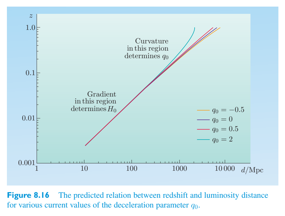
q 0.q 0。
Relating observations to the FRW models将观测结果与 FRW 模型联系起来
In 1929 Edwin Hubble announced his discovery, based on a small sample of relatively nearby galaxies (all with z < 0.004), that redshift increased roughly in proportion to distance. Actually, he sowed the seeds of much future confusion by using the approximate Doppler formula, v = cz, to convert the redshifts into recession velocities and then expressing his finding in terms of an increase of recession velocity with distance, but redshift is what was actually measured. This publication is usually hailed as marking the discovery of the expansion of the Universe.1929 年,埃德温·哈勃 (埃德温·哈勃) 宣布了他的发现,基于相对较近的星系的小样本(所有 z < 0.004),红移大致与距离成正比增加。实际上,他通过使用近似多普勒公式 v = cz 将红移转换为退行速度,然后用退行速度随距离增加的形式来表达他的发现,从而播下了许多未来混乱的种子,但红移是实际测量到的。这份出版物通常被誉为标志着宇宙膨胀的发现。
Hubble himself was always very cautious about the interpretation of his findings, but he was aware of de Sitter’s 1917 paper about an expanding Universe, and he knew that de Sitter had suggested that systematic increases in observed redshifts would be a consequence. In fact, towards the end of his 1929 paper, Hubble said:哈勃本人对他的发现的解释总是非常谨慎,但他知道德西特 1917 年关于宇宙膨胀的论文,并且他知道德西特暗示观测到的红移的系统性增加将是其结果。事实上,哈勃在 1929 年论文的末尾说道:
The outstanding feature, however, is the possibility that the velocity–distance relation may represent the de Sitter effect, and hence that numerical data may be introduced into discussions of the general curvature of space.然而,突出的特点是速度-距离关系可能代表德西特效应,因此可以将数值数据引入空间一般曲率的讨论中。
Hubble E., (1929) A relation between distance and radial velocity among extra-galactic nebulae, Proc. of the National Academy of Sciences of the United States of America, Vol. 15, Issue 3, pp. 168–73哈勃 E.,(1929) 河外星云距离与径向速度之间的关系,Proc。美国国家科学院院士,卷。 15,第 3 期,第 168–73 页
Ironically, de Sitter was also cautious about the significance of the redshifts that he predicted in his empty Universe, describing the associated positive radial velocities as ‘spurious’. As a result, there continues to be a mild academic debate about who should really be credited as the ‘discoverer’ of cosmic expansion.具有讽刺意味的是,德西特对他在空荡荡的宇宙中预测的红移的重要性也持谨慎态度,将相关的正径向速度描述为“虚假”。因此,关于谁应该真正被认为是宇宙膨胀的“发现者”,学术界仍然存在温和的争论。
Among Hubble’s original sample of galaxies, the highest radial velocity that he found was not much more than 1000 \(\mathrm{km\,s^{-1}}\). As a result, his original findings were badly affected by peculiar velocities that are typically of the order of hundreds of \(\mathrm{km\,s^{-1}}\). Nonetheless, he had recognized the basic nature of cosmic expansion, and within a few years had extended his studies to more distant galaxies with sufficiently high recessional velocities that their peculiar velocities were relatively unimportant compared with the effect of the large-scale (Hubble) flow. Subsequent studies, by Hubble and many others, have confirmed these general findings and led to a consensus that for moderately nearby galaxies, the observed relationship between redshift and luminosity distance can be described as follows.在哈勃最初的星系样本中,他发现的最高径向速度不超过 1000 \(\mathrm{km\,s^{-1}}\)。因此,他最初的发现受到了通常在数百 \(\mathrm{km\,s^{-1}}\) 数量级的特殊速度的严重影响。尽管如此,他已经认识到宇宙膨胀的基本性质,并在几年内将他的研究扩展到更遥远的星系,这些星系具有足够高的退行速度,与大规模(哈勃)流动的影响相比,它们的特殊速度相对不重要。哈勃和其他许多人的后续研究证实了这些一般性发现,并达成了共识,即对于中等邻近的星系,观察到的红移和光度距离之间的关系可以描述如下。
Observed redshift–distance relation观测到的红移-距离关系
where, according to one recent estimate, H = 74.2 ± 3.6 \(\mathrm{km\,s^{-1}\,Mpc^{-1}}\). It is conventional to refer to the currently observed proportionality constant \(H_0\) as the Hubble constant, but note that we have deliberately tailored our notation so that the (observational) Hubble constant can be seen as the current value of the (theoretical) Hubble parameter \(H(t)\).其中,根据最近的一项估计,H = 74.2 ± 3.6 \(\mathrm{km\,s^{-1}\,Mpc^{-1}}\)。通常将当前观测到的比例常数 \(H_0\) 称为哈勃常数,但请注意,我们特意调整了我们的符号,以便(观测)哈勃常数可以被视为(理论)哈勃参数 \(H(t)\) 的当前值。
An acceptable SI unit of \(H_0\) is the inverse second (\(\mathrm{s^{-1}}\)), but it is traditional to quote the Hubble constant in units of \(\mathrm{km\,s^{-1}\,Mpc^{-1}}\), harking back to Hubble’s decision to present his results as a velocity–distance relation. Indeed, it’s still the case that when astronomers invoke Hubble’s law, they usually write it in the form v = \(H_0\) d, despite the potential ambiguity of v and d.\(H_0\) 可接受的 SI 单位是秒的倒数 (\(\mathrm{s^{-1}}\)),但传统上以 \(\mathrm{km\,s^{-1}\,Mpc^{-1}}\) 为单位引用哈勃常数,这让人回想起哈勃决定将其结果表示为速度-距离关系。事实上,当天文学家援引哈勃定律时,他们通常将其写成 v = \(H_0\) d 的形式,尽管 v 和 d 可能存在歧义。
As data have accumulated, it has become increasingly clear that there are indeed deviations from the simple linear relation between redshift and luminosity distance. However, much of the evidence relates to observations of distant supernovae and involves sources with redshifts between 0.5 and 1. As a result, the approximate treatment that led to the deceleration parameter is not particularly useful. For that reason the use of the deceleration parameter has fallen into disfavour and has been replaced by other methods that we shall take up in the next subsection.随着数据的积累,越来越清楚的是,红移和光度距离之间的简单线性关系确实存在偏差。然而,许多证据与对遥远超新星的观测有关,并且涉及红移在 0.5 到 1 之间的源。因此,导致减速参数的近似处理并不是特别有用。因此,减速参数的使用已不再受欢迎,并已被我们将在下一小节中讨论的其他方法所取代。
8.4.2 Density parameters and the age of the Universe8.4.2 密度参数和宇宙年龄
We saw in Subsection 8.3.3 that we could specify the Friedmann equations relevant to a particular FRW model by giving the current values of three density parameters, \(\Omega_{m,0}\), \(\Omega_{r,0}\) and \(\Omega_{\Lambda,0}\), and we were able to specify a particular solution of those equations by imposing an appropriate boundary condition such as the value of \(R(t)\) at time \(t_0\). In practice the condition most often used is the current value of the Hubble parameter \(H_0\). The value (+1, 0 or − 1) of the curvature parameter k does not need to be specified because it is determined by the sign of \(\Omega_0\) − 1, where \(\Omega_0\) = \(\Omega_{m,0}\) + \(\Omega_{r,0}\) + \(\Omega_{\Lambda,0}\). So the set of parameters (\(\Omega_{m,0}\), \(\Omega_{r,0}\), \(\Omega_{\Lambda,0}\), \(H_0\)) specifies a particular FRW model with a specific expansion history and, in the case that it starts with a Big Bang, a definite age at time \(t_0\).我们在第 8.3.3 小节中看到,我们可以通过给出三个密度参数 \(\Omega_{m,0}\)、\(\Omega_{r,0}\) 和 \(\Omega_{\Lambda,0}\) 的当前值来指定与特定 FRW 模型相关的弗里德曼方程,并且我们能够通过施加适当的边界条件(例如 \(R(t)\) 在时间 \(t_0\) 时的值)来指定这些方程的特定解。在实践中,最常用的条件是哈勃参数 \(H_0\) 的当前值。不需要指定曲率参数 k 的值(+1、0 或 − 1),因为它由 \(\Omega_0\) − 1 的符号确定,其中 \(\Omega_0\) = \(\Omega_{m,0}\) + \(\Omega_{r,0}\) + \(\Omega_{\Lambda,0}\)。因此,参数集(\(\Omega_{m,0}\)、\(\Omega_{r,0}\)、\(\Omega_{\Lambda,0}\)、\(H_0\))指定了具有特定扩展历史的特定 FRW 模型,并且在它以大爆炸开始的情况下,指定了时间 \(t_0\) 的确定年龄。
In such a Universe the Friedmann equations can be used to supply a direct but complicated link between the co-moving coordinate of any source and the redshift of radiation from that source when it arrives at the origin at time \(t_0\). The model will also relate the co-moving coordinate of the source to its luminosity distance at time \(t_0\). Thus, provided that Hubble’s constant is known, it is possible to acquire information about the current values of the cosmic density parameters from measurements of redshift and luminosity distance.在这样的宇宙中,弗里德曼方程可用于在任何源的共动坐标与来自该源的辐射在时间 \(t_0\) 到达原点时的红移之间提供直接但复杂的联系。该模型还将源的共动坐标与其在时间 \(t_0\) 的光度距离相关联。因此,只要已知哈勃常数,就可以通过红移和光度距离的测量来获取有关宇宙密度参数当前值的信息。
In fact, there are several other ways of obtaining information about these parameters, particularly through detailed measurements of the anisotropies in the CMBR. We shall not pursue those here since they are discussed in detail in the companion volume on observational cosmology. We shall, however, note that as a result of a wide range of cosmological studies, primarily but not exclusively based on observations of the CMBR, there is now widespread agreement that the following set of parameter values provides a reasonable description of the large-scale features of our Universe.事实上,还有其他几种方法可以获取有关这些参数的信息,特别是通过详细测量 CMBR 中的各向异性。我们不会在这里追究这些问题,因为它们在观测宇宙学的姊妹篇中进行了详细讨论。然而,我们应该注意到,作为广泛的宇宙学研究的结果,主要但不完全基于 CMBR 的观测,现在人们普遍认为以下一组参数值提供了对我们宇宙的大尺度特征的合理描述。
Key cosmological parameters关键宇宙学参数
H = 74.2 ± 3.6 \(\mathrm{km\,s^{-1}\,Mpc^{-1}}\).H = 74.2 ± 3.6 \(\mathrm{km\,s^{-1}\,Mpc^{-1}}\)。
The implication is that the total density parameter is close to 1, so the Universe has a nearly flat spatial geometry with \(k = 0\) and a total density that is close to the 10 − 26 \(\mathrm{kg\,m^{-3}}\). current critical density \(\rho\) = 3 \(H^{2}\)/(8 πG), roughly 1 ×这意味着总密度参数接近 1,因此宇宙具有接近平坦的空间几何形状 \(k = 0\) 和接近 10 − 26 \(\mathrm{kg\,m^{-3}}\) 的总密度。电流临界密度 \(\rho\) = 3 \(H^{2}\)/(8 πG),大约 1 ×
This is an accelerating Universe of the kind that we discussed earlier. It started with a Big Bang, and light reaching us now (at time \(t_0\)) with redshift z can be shown to have been emitted at time这是我们之前讨论过的那种加速宇宙。它始于大爆炸,现在到达我们的光(在时间 \(t_0\)),红移 z 可以被证明是在时间发出的
so, the current age of the Universe, \(t_0\) (corresponding to所以,宇宙当前的年龄,\(t_0\)(对应于
With the currently favoured key values for the various parameters, this indicates a value for t of about \(13.7\times10^{9}\) years.根据目前青睐的各种参数的关键值,这表明 t 的值约为 \(13.7\times10^{9}\) 年。
As observational data improve, it will be interesting to see if these values continue to be upheld and if the use of a FRW cosmological model continues to be regarded as appropriate.随着观测数据的改进,看看这些价值观是否继续得到维护,以及 FRW 宇宙学模型的使用是否继续被认为是适当的,将会很有趣。
8.4.3 Horizons and limits8.4.3 范围和限制
We end with a short discussion of two diagrams that provide a general view of some general observational features of the kind of expanding, accelerating FRW model that is currently thought to describe our Universe. The diagrams are complicated and will repay detailed study. They are shown as Figures 8.17 and 8.18, and are based on diagrams produced by Mark Whittle of the University of Virginia, though they are also strongly related to diagrams published by C. H. Lineweaver and T. M. Davis in Publications of the Astronomical Society of Australia, vol. 21, pages 97–109 (2004).最后我们对两张图进行了简短的讨论,这两张图提供了目前被认为描述我们宇宙的膨胀、加速 FRW 模型的一些一般观测特征的总体视图。图表很复杂,需要详细研究。它们如图 8.17 和 8.18 所示,基于弗吉尼亚大学的 Mark Whittle 制作的图表,尽管它们也与 C. H. Lineweaver 和 T. M. Davis 在澳大利亚天文学会出版物 (Publications of the Astronomical Society of Australia) 第 1 卷中发表的图表密切相关。 21,第 97-109 页(2004 年)。
the current value of the scale factor. (We shall have more to say about these when we consider Figure 8.18.)尺度因子的当前值。 (当我们考虑图 8.18 时,我们将对这些有更多的讨论。)
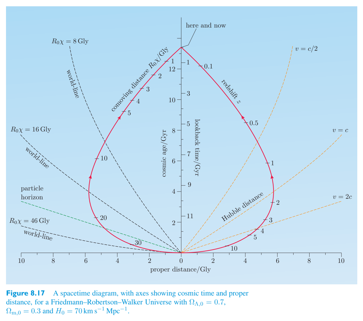
The curved black lines originating at (0, 0) that cut across the left-hand side of the past lightcone are the world-lines of ‘galaxies’ (or more accurately, fundamental observers) that travel along geodesics of the Robertson–Walker spacetime as they fall freely under the gravitational influence of the matter and dark energy that shape that spacetime. Each of these world-lines is marked with the co-moving distance of the corresponding ‘galaxy’. Also shown cutting across the left half of the past lightcone is a green line called the particle horizon. This represents the c from the (0, 0) event. At location in spacetime of a signal that travels with speed any cosmic time t, that line marks the location of the most distant object that can be observed. In this sense the particle horizon is the edge of the observable Universe. Currently the particle horizon is at a proper distance of about 46 billion light-years, though that is too far out to be shown on the diagram. Also shown crossing the left side of the diagram immediately below the particle horizon, is the world-line of a galaxy that is currently on the particle horizon. Up until now that galaxy has been outside the observable Universe. It is only now entering the observable Universe as the particle horizon moves outwards.起源于 (0, 0) 的黑色弯曲线穿过过去光锥的左侧,是“星系”(或更准确地说,基本观察者)的世界线,它们沿着罗伯逊-沃克时空的测地线行进,因为它们在塑造时空的物质和暗能量的引力影响下自由落体。每条世界线都标有相应“星系”的共动距离。图中还显示一条绿线穿过过去光锥的左半部分,称为粒子视界。这表示来自 (0, 0) 事件的 c。在以任何宇宙时间 t 的速度传播的信号的时空位置处,该线标记了可以观测到的最远物体的位置。从这个意义上说,粒子视界是可观测宇宙的边缘。目前,粒子视界的固有距离约为 460 亿光年,尽管这个距离太远而无法在图表中显示。还显示在粒子视界正下方穿过图左侧的,是当前位于粒子视界上的星系的世界线。到目前为止,该星系一直处于可观测宇宙之外。随着粒子视界向外移动,它现在才进入可观测的宇宙。
There is a second horizon, called the cosmological event horizon that is not shown on the diagram. This represents the past lightcone for observers at our position infinitely far in the future. It separates events that we might observe at some finite time from those that we will never be able to see, no matter how long we wait. That ultimate limit of observability is at about 60 billion light-years. No event that occurs beyond that event horizon will ever be seen from our location.还有第二个视界,称为宇宙事件视界,图中未显示。对于无限遥远的未来我们所在位置的观察者来说,这代表了过去的光锥。它将我们在某个有限时间内可能观察到的事件与无论我们等待多久都永远无法看到的事件区分开来。可观测性的最终极限约为 600 亿光年。从我们的位置看不到发生在事件视界之外的任何事件。
Another set of curves cuts across the right-hand half of the past lightcone. These lines connect points at which the Hubble flow has a specific proper radial velocity relative to fundamental observers on the vertical axis (i.e. us). Note in particular the middle (orange) line marked Hubble distance. This shows the proper distance at which an object participating in the Hubble flow would have a proper radial velocity of c. Note in particular that for the galaxies that we see now (i.e. those at the events that make up the past lightcone), all those with a redshift greater than about 1.5 are receding at a proper radial speed that is greater than c. All those with redshift less than 1.5 are receding at a sub-light speed. These ‘faster-than-light’ proper speeds are not in any way in conflict with the special relativistic prohibition on faster-than-light signals, because they are not carrying information between observers at faster-than-light speeds; rather, they concern the speed at which observers are being separated by the expansion of the Universe. Although it cannot be easily seen from the diagram, in order for an object to be receding from us at the speed of light, it would currently have to be at a proper distance of about 15 billion light-years.另一组曲线穿过过去光锥的右半部分。这些线联络哈勃流相对于垂直轴(即我们)上的基本观察者具有特定的适当径向速度的点。特别注意标记哈勃距离的中间(橙色)线。这显示了参与哈勃流的物体具有固有径向速度 c 的固有距离。特别注意,对于我们现在看到的星系(即构成过去光锥的事件中的星系),所有红移大于约 1.5 的星系都以大于 c 的适当径向速度后退。所有红移小于 1.5 的物体都以亚光速后退。这些“超光速”的固有速度与特殊相对论对超光速信号的禁令没有任何冲突,因为它们不会以超光速在观察者之间携带信息;相反,它们关注的是观察者因宇宙膨胀而分开的速度。虽然从图中不容易看出,但要让一个物体以光速远离我们,目前它的固有距离必须约为 150 亿光年。
Figure 8.18 shows essentially the same information but presents it using differently scaled axes. The horizontal axis now shows co-moving distance \(R(t_0)\) \(\chi\), while the vertical axis uses a variable called conformal time that, when combined with the use of co-moving distance, has the effect of making the past lightcone take on a form that is familiar in the flat spacetime of special relativity. The world-lines of galaxies are now simple vertical lines, reflecting their fixed co-moving coordinates. The definition of co-moving distance ensures that it is equal to the present value of the proper distance.图 8.18 显示了基本相同的信息,但使用不同比例的轴来呈现。横轴现在显示同移距离 \(R(t_0)\) \(\chi\),而纵轴使用称为共形时间的变量,当与同移距离结合使用时,具有使过去的光锥呈现狭义相对论平坦时空中熟悉的形式的效果。星系的世界线现在是简单的垂直线,反映了它们固定的共动坐标。共动距离的定义确保它等于固有距离的现值。
distance, for a 70 \(\mathrm{km\,s^{-1}\,Mpc^{-1}}\). The past and world-lines of fundamental emitted at a very small proper distance, less than 0.1 billion light-years but would currently be at a co-moving distance of about 45 billion light-years, close to the particle horizon.距离,70 \(\mathrm{km\,s^{-1}\,Mpc^{-1}}\)。过去和世界的基本线在非常小的固有距离(不到 1 亿光年)处发射,但目前的共动距离约为 450 亿光年,接近粒子视界。
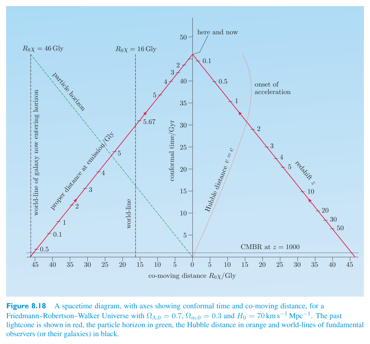
Exercise 8.11 Figure 8.1 and more particularly Figure练习 8.11 图 8.1 以及更具体的图
8.2 showed information8.2 显示信息
about the large-scale distribution of galaxies and quasars that extended to distances of order 10 billion light-years, yet Figure 8.17 indicates that we do not receive any signals from events at proper distances greater than about 5 billion light-years. Comment on this apparent inconsistency.关于星系和类星体的大规模分布,其距离延伸到 100 亿光年量级,但图 8.17 表明,我们没有收到任何来自距离大于约 50 亿光年的固有距离的事件的信号。对这种明显的不一致发表评论。
Exercise 8.12 To complete your work in this book,练习8.12 为了完成本书中的作业,
summarize the historical development of the Friedmann–Robertson–Walker models for the Universe.总结弗里德曼-罗伯逊-沃克宇宙模型的历史发展。
Summary of Chapter 8第 8 章总结
1. A starting assumption of modern relativistic cosmology1. 现代相对论宇宙学的起始假设
is that Einstein’s original (unmodified) field equations of general relativity can be applied to the Universe as a whole, provided that a possible contribution from dark energy is included. We may then speak interchangeably of a Universe characterized by a cosmological constant \(\Lambda\) or one in which there is a dark energy contribution of density \(\rho\) and (negative) pressure \(p = -\rho c^2 = -\Lambda c^4/(8\pi G)\). \(\Lambda\)爱因斯坦的原始(未经修改的)广义相对论场方程可以应用于整个宇宙,前提是包括暗能量的可能贡献。然后,我们可以互换地谈论以宇宙学常数 \(\Lambda\) 为特征的宇宙,或者其中存在密度 \(\rho\) 和(负)压力 \(p = -\rho c^2 = -\Lambda c^4/(8\pi G)\) 的暗能量贡献的宇宙。 \(\Lambda\)
2. According to the cosmological principle, at any given2. 根据宇宙学原理,在任意给定的情况下
time, and on a sufficiently large scale, the Universe is homogeneous (i.e. the same everywhere) and isotropic (i.e. the same in all directions). This is supported by a range of evidence, including the low level of intrinsic anisotropies in the cosmic microwave background radiation.在足够大的范围内,宇宙是均匀的(即各处相同)和各向同性的(即所有方向都相同)。这得到了一系列证据的支持,包括宇宙微波背景辐射中低水平的固有各向异性。
3. According to the Weyl postulate, in cosmic spacetime3. 根据外尔假设,在宇宙时空中
there exists a set of privileged fundamental observers whose world-lines form a smooth bundle of time-like geodesics. These geodesics never meet at any event, apart perhaps from an initial singularity in the past and/or a final singularity in the future. The motion of the Earth relative to the frame of a local fundamental observer can be deduced from the dipole anisotropy in the CMBR.存在着一组享有特权的基本观察者,他们的世界线形成了一束光滑的类似时间的测地线。这些测地线在任何情况下都不会相遇,除了过去的初始奇点和/或未来的最终奇点之外。地球相对于当地基本观测者坐标系的运动可以从 CMBR 中的偶极子各向异性推断出来。
4. The Robertson–Walker metric that describes a homogeneous4. 描述同构的罗伯逊-沃克度规
and isotropic spacetime is各向同性时空是
where t is the cosmic time, r, \(\theta\) and \(\phi\) are co-moving spherical coordinates, \(R(t)\) is the cosmic scale factor, and k is the spatial curvature parameter.其中 t 是宇宙时间,r、\(\theta\) 和 \(\phi\) 是共动球面坐标,\(R(t)\) 是宇宙尺度因子,k 是空间曲率参数。
5. In Robertson–Walker spacetime, proper distance \(\sigma\)5. 在罗伯逊-沃克时空中,固有距离 \(\sigma\)
(t) (as measured by a line of stationary rulers at some fixed cosmic time) is related to co-moving(t)(在某个固定的宇宙时间通过一排静止的标尺测量)与共动有关
leading to the relations导致关系
6. A further consequence at any time t is the exact relationship6. 任何时间 t 的进一步结果是精确关系
where d p represents the proper distance between two fundamental observers (or their galaxies), v p represents the proper radial velocity at which they are separating, and \(H(t)\) is the Hubble parameter, defined by其中 d p 表示两个基本观测者(或其星系)之间的固有距离,v p 表示它们分离时的适当径向速度,\(H(t)\) 是哈勃参数,定义为
7. The space-like hypersurfaces of a Robertson–Walker spacetime may be7. 罗伯逊-沃克时空的类空间超曲面可以是
described as open, flat or closed (and unbounded) according to the value of the curvature parameter k and the corresponding total volume of space, which may be infinite or finite.根据曲率参数 k 的值和相应的空间总体积(可以是无限的或有限的)被描述为开放、平坦或封闭(且无界)。
8. In homogeneous and isotropic cosmological models, where the contents of8. 在均匀和各向同性宇宙学模型中,其中
spacetime are represented by ideal fluids corresponding to matter, radiation and the source of dark energy, the uniform cosmic density \(\rho(t)\) and pressure \(p(t)\) are specified at time t = \(t_0\) by the quantities \(\rho_{m,0}\), \(\rho_{r,0}\) and \(\rho\) (and the appropriate equations of state linking them to pressure). Given these three values, the cosmic density and pressure at any other cosmic time can be determined, provided that the cosmic scale factor \(R(t)\) is known as an explicit function of cosmic time.时空由对应于物质、辐射和暗能量源的理想流体表示,均匀宇宙密度 \(\rho(t)\) 和压力 \(p(t)\) 在时间 t = \(t_0\) 时由量 \(\rho_{m,0}\)、\(\rho_{r,0}\) 和 \(\rho\)(以及将它们与压力联系起来的适当状态方程)指定。给定这三个值,只要宇宙尺度因子 \(R(t)\) 已知为宇宙时间的显式函数,就可以确定任何其他宇宙时间的宇宙密度和压力。
9. The evolution of the cosmic scale factor is determined by the Friedmann9. 宇宙尺度因子的演化由弗里德曼方程决定
equations方程
10. In practical applications, the Friedmann equations take the form10. 在实际应用中,弗里德曼方程的形式为
11. In flat space (\(k = 0\)), single-component models dominated respectively by11. 在平坦空间(\(k = 0\))中,单分量模型分别占主导地位
matter, radiation and dark energy, the cosmic scale factor evolves as follows:物质、辐射和暗能量,宇宙尺度因子的演变如下:
de Sitter model德西特模型
flat, pure radiation model平坦、纯辐射模型
Einstein–de Sitter model爱因斯坦-德西特模型
12. A relativistic cosmological model based on the Robertson–Walker12. 基于罗伯逊-沃克的相对论宇宙学模型
metric with a scale factor determined by the Friedmann equations is known as a Friedmann–Robertson–Walker (FRW) model. When specifying a general FRW model it is conventional to express each of the densities as a fraction of the critical density \(\rho = 3H^2(t)/(8\pi G)\). These fractional densities are called density parameters and are defined as follows:具有由弗里德曼方程确定的尺度因子的度规称为弗里德曼-罗伯逊-沃克 (FRW) 模型。当指定通用 FRW 模型时,通常将每个密度表示为临界密度 \(\rho = 3H^2(t)/(8\pi G)\) 的一部分。这些分数密度称为密度参数,定义如下:
13. The Friedmann equations imply that13. 弗里德曼方程意味着
if \(\Omega\) + \(\Omega\) + \(\Omega\) < 1, then k < 0 and space如果 \(\Omega\) + \(\Omega\) + \(\Omega\) < 1,则 k < 0 并且空格
if \(\Omega\) + \(\Omega\) + \(\Omega\) = 1, then \(k = 0\) and space如果 \(\Omega\) + \(\Omega\) + \(\Omega\) = 1,则 \(k = 0\) 和空格
if \(\Omega\) + \(\Omega\) + \(\Omega\) > 1, then k > 0 and space如果 \(\Omega\) + \(\Omega\) + \(\Omega\) > 1,则 k > 0 且空格
14. A quantitative measure of redshift is14. 红移的定量测量是
In a Friedmann–Robertson–Walker model, observed redshift is related to the scale factor by在弗里德曼-罗伯逊-沃克模型中,观测到的红移与尺度因子的关系为
15. The luminosity distance of an isotropically radiating15. 各向同性辐射的光度距离
source is defined by源定义为
and is related to redshift at small z by the approximate relation并通过近似关系与小 z 处的红移相关
where \(H_0\) and q 0 represent the current values of the Hubble and deceleration parameters. To a first approximation this is consistent with Hubble’s (observational) law (v = \(H_0\) d) and allows the observed Hubble constant to be identified with \(H(t_0)\).其中 \(H_0\) 和 q 0 表示哈勃和减速参数的当前值。初步近似,这与哈勃(观测)定律 (v = \(H_0\) d) 一致,并且允许将观测到的哈勃常数与 \(H(t_0)\) 进行识别。
16. Currently observed values of the key cosmological16. 目前观测到的关键宇宙学值
parameters include参数包括
H = 74.2 ± 3.6 \(\mathrm{km\,s^{-1}\,Mpc^{-1}}\).H = 74.2 ± 3.6 \(\mathrm{km\,s^{-1}\,Mpc^{-1}}\)。
The implication is that the total density parameter is close to 1, so the Universe has a nearly flat spatial geometry with \(k = 0\) and a total density that is close to \(1\times10^{-26}\) \(\mathrm{kg\,m^{-3}}\). Such a Universe originated with a Big Bang, is accelerating its expansion and has an expansion age of about这意味着总密度参数接近于1,因此宇宙具有接近平坦的空间几何形状,为\(k = 0\),总密度接近于\(1\times10^{-26}\) \(\mathrm{kg\,m^{-3}}\)。这样的宇宙起源于大爆炸,正在加速膨胀,膨胀年龄约为
13.7 billion years.137亿年。
Appendix附录
Table A.1 Common SI unit conversions and derived units Quantity speed acceleration angular speed angular acceleration rad \(\mathrm{s^{-2}}\) linear momentum angular momentum kg \(m^{2}\) \(\mathrm{s^{-1}}\) force energy power pressure frequency charge potential difference volt (V) electric field magnetic field表 A.1 常用 SI 单位换算及导出单位数量速度加速度角速度角加速度 rad \(\mathrm{s^{-2}}\) 线动量角动量 kg \(m^{2}\) \(\mathrm{s^{-1}}\) 力能量功率压力频率电荷电势差伏特(V) 电场磁场
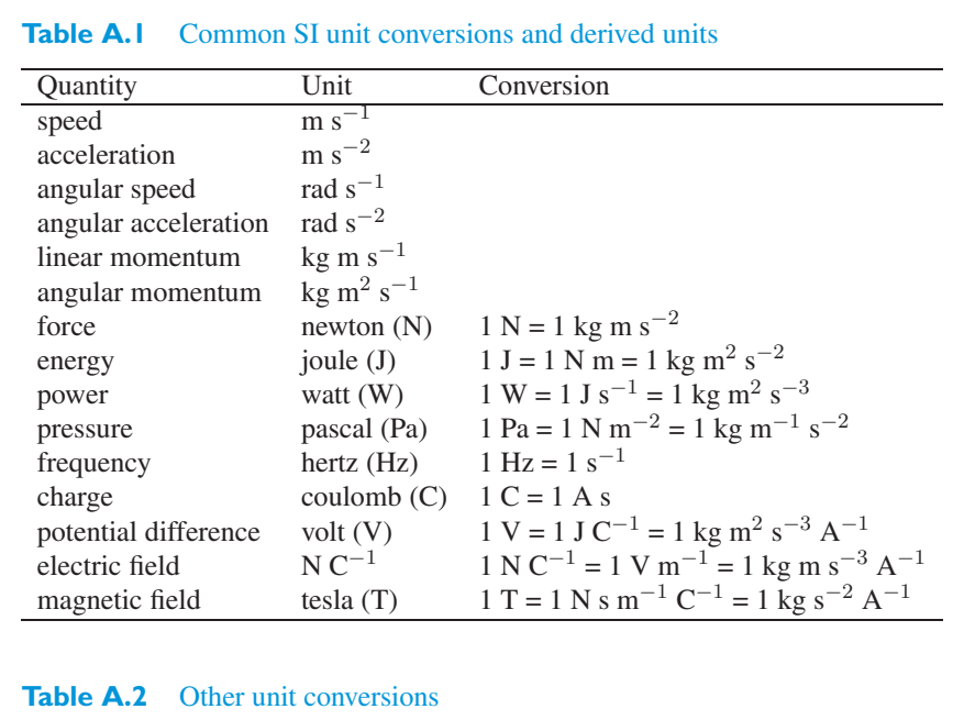
Quantity Unit Conversion \(\mathrm{m\,s^{-1}}\) speed \(\mathrm{m\,s^{-2}}\) acceleration rad \(\mathrm{s^{-1}}\) angular speed angular acceleration rad \(\mathrm{s^{-2}}\) linear momentum \(\mathrm{kg\,m\,s^{-1}}\) angular momentum kg \(m^{2}\) \(\mathrm{s^{-1}}\) force newton (N) 1 N = 1 \(\mathrm{kg\,m\,s^{-2}}\) energy joule (J) 1 J = 1 N m = 1 kg \(m^{2}\) \(\mathrm{s^{-2}}\) power watt (W) 1 W = 1 \(\mathrm{J\,s^{-1}}\) = 1 kg \(m^{2}\) s − 3 1 Pa = 1 \(\mathrm{N\,m^{-2}}\) = 1 \(\mathrm{kg\,m^{-1}\,s^{-2}}\) pressure pascal (Pa) frequency hertz (Hz) 1 Hz = 1 \(\mathrm{s^{-1}}\) charge coulomb (C) 1 C = 1 A s potential difference volt (V) 1 V = 1 J \(\mathrm{C^{-1}}\) = 1 kg \(m^{2}\) s − 3 \(\mathrm{A^{-1}}\) N \(\mathrm{C^{-1}}\) electric field 1 N \(\mathrm{C^{-1}}\) = 1 V \(\mathrm{m^{-1}}\) = 1 kg m s − 3 \(\mathrm{A^{-1}}\) magnetic field tesla (T) 1 T = 1 N s \(\mathrm{m^{-1}}\) \(\mathrm{C^{-1}}\) = 1 kg \(\mathrm{s^{-2}}\) \(\mathrm{A^{-1}}\)数量单位换算 \(\mathrm{m\,s^{-1}}\) 速度 \(\mathrm{m\,s^{-2}}\) 加速度 rad \(\mathrm{s^{-1}}\) 角速度角加速度 rad \(\mathrm{s^{-2}}\) 线动量 \(\mathrm{kg\,m\,s^{-1}}\) 角动量 kg \(m^{2}\) \(\mathrm{s^{-1}}\) 力牛顿 (N) 1 N = 1 \(\mathrm{kg\,m\,s^{-2}}\) 能量焦耳 (J) 1 J = 1 N m = 1 kg \(m^{2}\) \(\mathrm{s^{-2}}\) 次方瓦特 (W) 1 W = 1 \(\mathrm{J\,s^{-1}}\) = 1 kg \(m^{2}\) s − 3 1 Pa = 1 \(\mathrm{N\,m^{-2}}\) = 1 \(\mathrm{kg\,m^{-1}\,s^{-2}}\) 压力帕斯卡 (Pa) 频率赫兹 (Hz) 1 Hz = 1 \(\mathrm{s^{-1}}\) 电荷库仑 (C) 1 C = 1 A s 电势差伏特 (V) 1 V = 1 J \(\mathrm{C^{-1}}\) = 1 kg \(m^{2}\) s − 3 \(\mathrm{A^{-1}}\) N \(\mathrm{C^{-1}}\) 电场 1 N \(\mathrm{C^{-1}}\) = 1 V \(\mathrm{m^{-1}}\) = 1 kg m s − 3 \(\mathrm{A^{-1}}\) 磁场 tesla (T) 1 T = 1 N s \(\mathrm{m^{-1}}\) \(\mathrm{C^{-1}}\) = 1 kg \(\mathrm{s^{-2}}\) \(\mathrm{A^{-1}}\)
Table A.2 Other unit conversions wavelength 1 nanometre (nm) = 10\(\text{\AA}\) = 10 − 9 m 1 kg = \(8.99\times10^{16}\) J/\(c^2\) (c in \(\mathrm{m\,s^{-1}}\)) 1 ångström = 0.1 nm = 10 − 10 m angular measure 1 ◦ = 60 arcmin = 3600 arcsec 1 ◦ = 0.01745 radian 1 radian = 57.30 ◦ temperature absolute zero: 0 K = − 273.15 ◦ C 0 ◦ C = 273.15 K spectral flux density 1 jansky (Jy) = 10 − 26 W \(\mathrm{m^{-2}}\) Hz − 1 1 barn = 10 − 28 \(m^{2}\) 1 W \(\mathrm{m^{-2}}\) Hz − 1 = \(10^{26}\) Jy cgs units 1 erg = 10 − 7 J 1 dyne = 10 − 5 N 1 gauss = 10 − 4 \(T^{1}\) emu = 10 C表 A.2 其他单位换算波长 1 纳米 (nm) = 10\(\text{\AA}\) = 10 − 9 m 1 kg = \(8.99\times10^{16}\) J/\(c^2\) (c in \(\mathrm{m\,s^{-1}}\)) 1 ångström = 0.1 nm = 10 − 10 m 角度测量 1° = 60 arcmin = 3600 arcsec 1° = 0.01745弧度 1 弧度 = 57.30 ° 温度绝对零: 0 K = − 273.15 ° C 0 ° C = 273.15 K 光谱通量密度 1 jansky (Jy) = 10 − 26 W \(\mathrm{m^{-2}}\) Hz − 1 1 barn = 10 − 28 \(m^{2}\) 1 W \(\mathrm{m^{-2}}\) Hz − 1 = \(10^{26}\) Jy cgs 单位 1 erg = 10 − 7 J 1 达因 = 10 − 5 N 1 高斯 = 10 − 4 \(T^{1}\) emu = 10 C
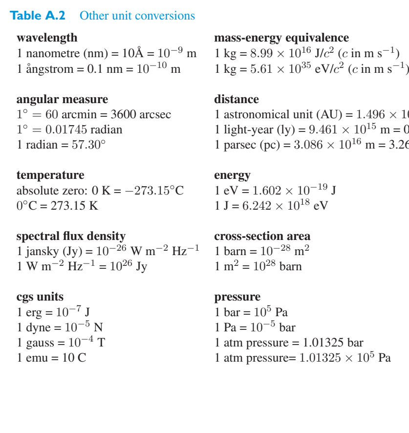
wavelength mass-energy equivalence 1 nanometre (nm) = 10\(\text{\AA}\) = 10 − 9 m 1 kg = \(8.99\times10^{16}\) J/\(c^2\) (c in \(\mathrm{m\,s^{-1}}\)) 1 kg = \(5.61\times10^{35}\) eV/\(c^2\) (c in \(\mathrm{m\,s^{-1}}\)) 1 ångström = 0.1 nm = 10 − 10 m波长质能当量 1 纳米 (nm) = 10\(\text{\AA}\) = 10 − 9 m 1 kg = \(8.99\times10^{16}\) J/\(c^2\) (c in \(\mathrm{m\,s^{-1}}\)) 1 kg = \(5.61\times10^{35}\) eV/\(c^2\) (c in \(\mathrm{m\,s^{-1}}\)) 1 ångström = 0.1 nm = 10 − 10 m
angular measure distance 1 astronomical unit (AU) = \(1.496\times10^{11}\) 1 ◦ = 60 arcmin = 3600 arcsec m 1 ◦ = 0.01745 radian 1 light-year (ly) = \(9.461\times10^{15}\) m = 0.307 pc 1 radian = 57.30 ◦ 1 parsec (pc) = \(3.086\times10^{16}\) m = 3.26 ly角度测量距离 1 天文单位 (AU) = \(1.496\times10^{11}\) 1 ◦ = 60 arcmin = 3600 arcsec m 1 ◦ = 0.01745 弧度 1 光年 (ly) = \(9.461\times10^{15}\) m = 0.307 pc 1 弧度 = 57.30 ◦ 1 秒差距 (pc) = \(3.086\times10^{16}\) m = 3.26 ly
temperature energy 1 eV = \(1.602\times10^{-19}\) J absolute zero: 0 K = − 273.15 ◦ C 1 J = \(6.242\times10^{18}\) eV 0 ◦ C = 273.15 K温度能量 1 eV = \(1.602\times10^{-19}\) J 绝对零:0 K = − 273.15 ◦ C 1 J = \(6.242\times10^{18}\) eV 0 ◦ C = 273.15 K
spectral flux density cross-section area 1 jansky (Jy) = 10 − 26 W \(\mathrm{m^{-2}}\) Hz − 1 1 barn = 10 − 28 \(m^{2}\) 1 W \(\mathrm{m^{-2}}\) Hz − 1 = \(10^{26}\) Jy 1 \(m^{2}\) = \(10^{28}\) barn谱通量密度横截面积 1 jansky (Jy) = 10 − 26 W \(\mathrm{m^{-2}}\) Hz − 1 1 barn = 10 − 28 m 2 1 W \(\mathrm{m^{-2}}\) Hz − 1 = \(10^{26}\) Jy 1 m 2 = \(10^{28}\) barn
cgs units pressure 1 erg = 10 − 7 J 1 bar = 10 5 Pa 1 dyne = 10 − 5 N 1 Pa = 10 − 5 bar 1 gauss = 10 − 4 \(T^{1}\) atm pressure = 1.01325 bar 1 atm pressure= \(1.01325\times10^{5}\) Pa 1 emu = 10 Ccgs 单位压力 1 erg = 10 − 7 J 1 bar = 10 5 Pa 1 dyne = 10 − 5 N 1 Pa = 10 − 5 bar 1 高斯 = 10 − 4 \(T^{1}\) atm 压力 = 1.01325 bar 1 atm 压力= \(1.01325\times10^{5}\) Pa 1 emu = 10 C
Table A.3 Constants Name of constant Fundamental constants gravitational constant Boltzman constant speed of light in vacuum Planck constant fine structure constant Stefan-Boltzman constant Thomson cross-section permittivity of free space permeability of free space Particle constants charge of proton charge of electron electron rest mass proton rest mass neutron rest mass atomic mass unit Astronomical constants mass of the Sun radius of the Sun luminosity of the sun mass of the Earth radius of the Earth mass of Jupiter radius of Jupiter astronomical unit light-year parsec Hubble constant age of Universe critical density dark energy density parameter matter density parameter baryonic matter density parameter non-baryonic matter density parameter \(\Omega\) curvature density parameter deceleration parameter表 A.3 常数名称基本常数玻尔兹曼真空光速普朗克常数精细结构常数斯特凡-玻尔兹曼常数汤姆逊截面介电常数自由空间磁导率自由空间磁导率粒子常数电子质子电荷电荷电子静止质量质子静止质量中子静止质量原子质量单位天文常数质量太阳半径太阳光度地球质量地球半径木星半径天文单位光年秒差距哈勃常数宇宙年龄临界密度暗能量密度参数物质密度参数重子物质密度参数非重子物质密度参数 \(\Omega\) 曲率密度参数减速参数
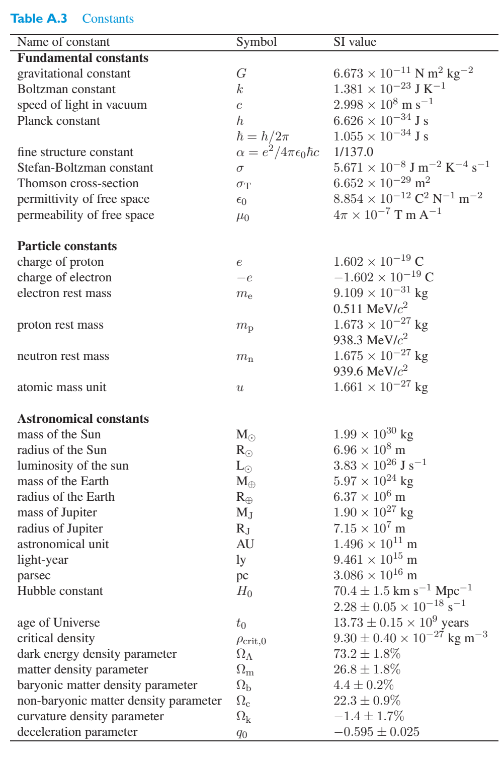
Name of constant Symbol SI value Fundamental constants常数名称符号 SI值基本常数
\(6.673\times10^{-11}\) N \(m^{2}\) kg − 2\(6.673\times10^{-11}\) N \(m^{2}\) 千克 − 2
gravitational constant万有引力常数
\(1.381\times10^{-23}\) \(\mathrm{J\,K^{-1}}\)\(1.381\times10^{-23}\) \(\mathrm{J\,K^{-1}}\)
Boltzman constant玻尔兹曼常数
\(2.998\times10^{8}\) \(\mathrm{m\,s^{-1}}\)\(2.998\times10^{8}\) 毫秒 − 1
speed of light in vacuum真空中的光速
\(6.626\times10^{-34}\) \(\mathrm{J\,s}\)\(6.626\times10^{-34}\) \(\mathrm{J\,s}\)
Planck constant普朗克常数
\(1.055\times10^{-34}\) \(\mathrm{J\,s}\)\(1.055\times10^{-34}\) \(\mathrm{J\,s}\)
\(\alpha\) = e 2/4 πh! c 1/137.0 fine structure constant\(\alpha\) = e 2/4 πh! c 1/137.0 精细结构常数
\(5.671\times10^{-8}\) \(\mathrm{J\,m^{-2}\,K^{-4}\,s^{-1}}\)\(5.671\times10^{-8}\) \(\mathrm{J\,m^{-2}\,K^{-4}\,s^{-1}}\)
Stefan-Boltzman constant斯特凡-玻尔兹曼常数
\(6.652\times10^{-29}\) \(m^{2}\)\(6.652\times10^{-29}\) \(m^{2}\)
Thomson cross-section汤姆逊截面
\(8.854\times10^{-12}\) \(\mathrm{C^2\,N^{-1}\,m^{-2}}\)\(8.854\times10^{-12}\) \(\mathrm{C^2\,N^{-1}\,m^{-2}}\)
permittivity of free space 4 \(\pi\) × 10 − 7 T m \(\mathrm{A^{-1}}\) permeability of free space自由空间介电常数 4 \(\pi\) × 10 − 7 T m \(\mathrm{A^{-1}}\) 自由空间磁导率
Particle constants粒子常数
\(1.602\times10^{-19}\) C\(1.602\times10^{-19}\) C
charge of proton − \(1.602\times10^{-19}\) C charge of electron质子电荷 − \(1.602\times10^{-19}\) C 电子电荷
\(9.109\times10^{-31}\) kg\(9.109\times10^{-31}\) 公斤
electron rest mass电子静止质量
0.511 MeV/\(c^2\)0.511兆伏/\(c^2\)
\(1.673\times10^{-27}\) kg\(1.673\times10^{-27}\) 公斤
proton rest mass质子静止质量
938.3 MeV/\(c^2\)938.3兆伏/\(c^2\)
\(1.675\times10^{-27}\) kg\(1.675\times10^{-27}\) 公斤
neutron rest mass中子静止质量
939.6 MeV/\(c^2\)939.6兆伏/\(c^2\)
\(1.661\times10^{-27}\) kg\(1.661\times10^{-27}\) 公斤
atomic mass unit原子质量单位
Astronomical constants天文常数
\(1.99\times10^{30}\) kg\(1.99\times10^{30}\) 公斤
mass of the Sun M)太阳质量 M)
\(6.96\times10^{8}\) m\(6.96\times10^{8}\) 米
radius of the Sun R)太阳半径 R)
\(3.83\times10^{26}\) \(\mathrm{J\,s^{-1}}\)\(3.83\times10^{26}\) \(\mathrm{J\,s^{-1}}\)
luminosity of the sun L太阳光度L
\(5.97\times10^{24}\) kg\(5.97\times10^{24}\) 公斤
mass of the Earth M ⊕地球质量 M ⊕
\(6.37\times10^{6}\) m\(6.37\times10^{6}\) 米
radius of the Earth R ⊕地球半径 R ⊕
\(1.90\times10^{27}\) kg\(1.90\times10^{27}\) 公斤
mass of Jupiter M木星质量 M
\(7.15\times10^{7}\) m\(7.15\times10^{7}\) 米
radius of Jupiter R木星半径 R
\(1.496\times10^{11}\) m\(1.496\times10^{11}\) 米
astronomical unit AU天文单位AU
\(9.461\times10^{15}\) m\(9.461\times10^{15}\) 米
light-year ly光年
\(3.086\times10^{16}\) m\(3.086\times10^{16}\) 米
parsec pc秒差距
70.4 ± 1.5 \(\mathrm{km\,s^{-1}\,Mpc^{-1}}\)70.4±1.5\(\mathrm{km\,s^{-1}\,Mpc^{-1}}\)
Hubble constant哈勃常数
2.28 ± \(0.05\times10^{-18}\) \(\mathrm{s^{-1}}\)2.28 ± \(0.05\times10^{-18}\) \(\mathrm{s^{-1}}\)
13.73 ± \(0.15\times10^{9}\) years13.73 ± \(0.15\times10^{9}\) 年
age of Universe宇宙年龄
9.30 ± \(0.40\times10^{-27}\) \(\mathrm{kg\,m^{-3}}\)9.30 ± \(0.40\times10^{-27}\) \(\mathrm{kg\,m^{-3}}\)
critical density dark energy density parameter matter density parameter baryonic matter density parameter non-baryonic matter density parameter \(\Omega\) curvature density parameter deceleration parameter临界密度暗能量密度参数物质密度参数重子物质密度参数非重子物质密度参数 \(\Omega\) 曲率密度参数减速参数
Solutions to exercises练习题解答
Exercise 1.1 A stationary particle in any laboratory on the Earth is actually练习 1.1 地球上任何实验室中的静止粒子实际上都是
subject to gravitational forces due to the Earth and the Sun. These help to ensure that the particle moves with the laboratory. If steps were taken to counterbalance these forces so that the particle was really not subject to any net force, then the rotation of the Earth and the Earth’s orbital motion around the Sun would carry the laboratory away from the particle, causing the force-free particle to follow a curving path through the laboratory. This would clearly show that the particle did not have constant velocity in the laboratory (i.e. constant speed in a fixed direction) and hence that a frame fixed in the laboratory is not an inertial frame. More realistically, an experiment performed using the kind of long, freely suspended pendulum known as a Foucault pendulum could reveal the fact that a frame fixed on the Earth is rotating and therefore cannot be an inertial frame of reference. An even more practical demonstration is provided by the winds, which do not flow directly from areas of high pressure to areas of low pressure because of the Earth’s rotation.受到地球和太阳的引力。这些有助于确保粒子随实验室移动。如果采取措施来平衡这些力,使粒子真正不受任何净力的影响,那么地球的自转和地球绕太阳的轨道运动将使实验室远离粒子,导致不受力的粒子沿着一条弯曲的路径穿过实验室。这清楚地表明粒子在实验室中不具有恒定速度(即在固定方向上的恒定速度),因此实验室中固定的框架不是惯性系。更现实的是,使用一种称为傅科摆的长的、自由悬挂的摆进行的实验可以揭示这样一个事实:固定在地球上的框架正在旋转,因此不能成为惯性参考系。风提供了更实际的证明,由于地球自转,风不会直接从高压区域流向低压区域。
Exercise 1.2 The Lorentz factor is \(\gamma(V)\) = 1/1 − \(V^{2}\)/\(c^2\).练习 1.2 洛伦兹因子为 \(\gamma(V)\) = 1/1 − \(V^{2}\)/\(c^2\)。
(a) If V = 0.1 c, then(a) 如果 V = 0.1 c,则
= 1.01 (to 3 s.f.).= 1.01(至 3 平方英尺)。
(b) If V = 0.9 c, then(b) 如果 V = 0.9 c,则
= 2.29 (to 3 s.f.).= 2.29(至 3 平方英尺)。
Note that it is often convenient to write speeds in terms of c instead of writing the values in \(\mathrm{m\,s^{-1}}\), because of the cancellation between factors of c.请注意,由于 c 因子之间的抵消,通常用 c 表示速度比用 \(\mathrm{m\,s^{-1}}\) 表示值更方便。
Exercise 1.3 The inverse of a 2 × 2 matrix M =练习 1.3 2 × 2 矩阵的逆 M =
is是
.。
Taking A = \(\gamma(V)\), B = − \(\gamma(V)\) V/c, C = − \(\gamma(V)\) V/c and D = \(\gamma(V)\), and noting that AD − BC = [\(\gamma(V)\)] 2 (1 − \(V^{2}\)/\(c^2\)) = 1, we have取 A = \(\gamma(V)\)、B = − \(\gamma(V)\) V/c、C = − \(\gamma(V)\) V/c 和 D = \(\gamma(V)\),并注意到 AD − BC = [\(\gamma(V)\)] 2 (1 − \(V^{2}\)/\(c^2\)) = 1,我们有
This is the correct form of the inverse Lorentz transformation matrix.这是洛伦兹逆变换矩阵的正确形式。
Exercise 1.4 First compute the Lorentz factor:练习1.4 首先计算洛伦兹因子:
Thus the measured lifetime is \(\Delta T = 5\)× 2.2/4 \(\mu\) s = 2.8 \(\mu\) s. Note that not all muons live for the same time; rather, they have a range of lifetimes. But a large group of muons travelling with a common speed does have a well-defined mean lifetime, and it is the dilation of this quantity that is easily demonstrated experimentally.因此,测得的寿命为 \(\Delta T = 5\)× 2.2/4 \(\mu\) s = 2.8 \(\mu\) s。请注意,并非所有 \(\mu\) 子都存在同一时间;相反,它们有一定的生命周期。但是,以共同速度行进的一大群\(\mu\)子确实具有明确定义的平均寿命,并且这个量的膨胀很容易通过实验证明。
Exercise 1.5 The alternative definition of length can’t be used in the rest frame练习1.5 长度的替代定义不能在静止坐标系中使用
of the rod as the rod does not move in its own rest frame. The proper length is therefore defined as before and related to the positions of the two events as observed in the rest frame. (This works, because event 1 and event 2 still occur at the end-points of the rod and the rod never moves in the rest frame \(S'\).)因为杆不在其自己的静止框架中移动。因此,正确的长度如前所述定义,并与在静止帧中观察到的两个事件的位置相关。 (这是可行的,因为事件 1 和事件 2 仍然发生在杆的端点处,并且杆永远不会在静止坐标系 \(S'\) 中移动。)
As before, it is helpful to write down all the intervals that are known in a table.和以前一样,在表格中写下所有已知的间隔会很有帮助。
Event S (laboratory) \(S'\) (rest frame)事件S(实验室)\(S'\)(休息架)
Intervals间隔
Relation to intervals (L/V, 0)与间隔的关系 (L/V, 0)
By examining the intervals, it can be seen that \(\Delta x\), \(\Delta t\) and \(\Delta x'\) are known. From the interval transformation rules, only Equation 1.33 relates the three known intervals. Substituting the known intervals into that equation gives L = \(\gamma(V)\)(0 − V (L/V)). In this way, length contraction is predicted as before:通过检查间隔,可以看出 \(\Delta x\)、\(\Delta t\) 和 \(\Delta x'\) 是已知的。从区间变换规则来看,只有方程 1.33 将三个已知区间联系起来。将已知区间代入该方程可得出 L = \(\gamma(V)\)(0 − V (L/V))。这样,长度收缩的预测就如之前一样:
Exercise 1.6 The received wavelength is less than the emitted wavelength. This means that the jet is approaching. We can therefore use Equation 1.42 provided that we change - the sign of V. Combining it with the formula f \(\lambda\) = c shows that \(\lambda'\) = \(\lambda\) (c − V)/(c + V). Squaring both sides and rearranging gives练习1.6 接收波长小于发射波长。这意味着喷气机正在接近。因此,只要我们改变 - V 的符号,我们就可以使用公式 1.42。将其与公式 f \(\lambda\) = c 相结合表明 \(\lambda'\) = \(\lambda\) (c − V)/(c + V)。将两边平方并重新排列得到
From this it follows that由此可见
so所以
thus因此
Substituting \(\lambda'\) = \(4483\times10^{-10}\) m and \(\lambda\) = \(5850\times10^{-10}\) m, the speed is found to be v = 0.26 c (to 2 s.f.).代入 \(\lambda'\) = \(4483\times10^{-10}\) m 和 \(\lambda\) = \(5850\times10^{-10}\) m,则速度为 v = 0.26 c(至 2 s.f.)。
Exercise 1.7 Let the spacestation be the origin of frame S, and the nearer of the练习 1.7 设空间站为 S 系的原点,且较近的
spacecraft the origin of frame \(S'\), which therefore moves with speed V = c/2 as measured in S. Let these two frames be in standard configuration. The velocity of the further of the two spacecraft, as observed in S, is then v = (3 c/4, 0, 0). It follows from the velocity transformation that the velocity of the further spacecraft as observed from the nearer will be \(v'\) = (\(v'\), 0, 0), where航天器的坐标系 \(S'\) 为原点,因此以 S 中测量的速度 V = c/2 移动。让这两个坐标系处于标准配置。在 S 中观测到的两个航天器中较远的一个的速度为 v = (3 c/4, 0, 0)。从速度变换可以看出,从较近的航天器观察到的较远的航天器的速度将为 \(v'\) = (\(v'\), 0, 0),其中
Exercise 1.8 \(\Delta x =\)(5 − 7) m = − 2 m and c \(\Delta t =\)(5 − 3) m = 2 m. Since the练习 1.8 \(\Delta x =\)(5 − 7) m = − 2 m 且 c \(\Delta t =\)(5 − 3) m = 2 m。自从
spacetime separation is (\(\Delta s\)) 2 = (c \(\Delta t\)) 2 − (\(\Delta x\)) 2 in this case, it follows that在这种情况下,时空间隔为 (\(\Delta s\)) 2 = (c \(\Delta t\)) 2 − (\(\Delta x\)) 2,由此得出
(\(\Delta s\)) 2 = (2 m) 2 − (2 m) 2 = 0. The value (\(\Delta s\)) 2 = 0 is permitted; it describes situations in which the two events could be linked by a light signal. In fact, any such separation is said to be light-like.(\(\Delta s\)) 2 = (2 m) 2 − (2 m) 2 = 0。 (\(\Delta s\)) 2 = 0 值是允许的;它描述了两个事件可以通过光信号联系起来的情况。事实上,任何这样的分离都被认为是类似光的。
Exercise 1.9 Start with (\(\Delta s'\)) 2 = (c \(\Delta t'\)) 2 − (\(\Delta x'\)) 2. The aim is to show that练习 1.9 从 (\(\Delta s'\)) 2 = (c \(\Delta t'\)) 2 − (\(\Delta x'\)) 2 开始。目的是证明
(\(\Delta s'\)) 2 = (\(\Delta s\)) 2.(\(\Delta s'\)) 2 = (\(\Delta s\)) 2。
Substitute \(\Delta x'\) = \(\gamma(\Delta x - V \Delta t)\) and c \(\Delta t'\) = \(\gamma(c \Delta t - V \Delta x/c)\) so that将 \(\Delta x'\) = \(\gamma(\Delta x - V \Delta t)\) 和 c \(\Delta t'\) = \(\gamma(c \Delta t - V \Delta x/c)\) 代入,使得
Cross terms involving \(\Delta x\) \(\Delta t\) cancel. Collecting common terms in \(c^2\) (\(\Delta t\)) 2 and (\(\Delta x\)) 2 gives涉及 \(\Delta x\) \(\Delta t\) 的交叉项取消。收集 \(c^2\) (\(\Delta t\)) 2 和 (\(\Delta x\)) 2 中的常用项得出
Finally, noting that γ 2 = [1 − \(V^{2}\)/\(c^2\)] − 1, there is a cancellation of terms, giving最后,注意到 γ 2 = [1 − \(V^{2}\)/\(c^2\)] − 1,项被取消,给出
thus showing that (\(\Delta s'\)) 2 = (\(\Delta s\)) 2.从而表明 (\(\Delta s'\)) 2 = (\(\Delta s\)) 2。
Exercise 1.10 Since (\(\Delta s\)) 2 = (c \(\Delta t\)) 2 − (\(\Delta l\)) 2, and (\(\Delta s\)) 2 is invariant, it练习1.10 由于 (\(\Delta s\)) 2 = (c \(\Delta t\)) 2 − (\(\Delta l\)) 2 并且 (\(\Delta s\)) 2 是不变的,因此
follows that all observers will find (c \(\Delta t\)) 2 = (\(\Delta s\)) 2 + (\(\Delta l\)) 2, where (\(\Delta l\)) 2 cannot be negative. Since (\(\Delta l\)) 2 = 0 in the frame in which the proper time is measured, it follows that no other observer can find a smaller value for the time between the events.由此可知,所有观察者都会发现 (c \(\Delta t\)) 2 = (\(\Delta s\)) 2 + (\(\Delta l\)) 2,其中 (\(\Delta l\)) 2 不能为负。由于在测量固有时间的帧中 (\(\Delta l\)) 2 = 0,因此没有其他观察者可以找到事件之间的时间的较小值。
Exercise 1.11 In Terra’s frame, Stella’s ship has velocity练习 1.11 在 Terra 的坐标系中,Stella 的船有速度
(v, v, v) = (− V, 0, 0). It follows from the velocity transformation that in Astra’s frame, the velocity of Stella’s ship will be (v \(x'\), 0, 0), where \(v'\) = (v − V)/(1 − v V/\(c^2\)). Taking v = − V gives(v, v, v) = (− V, 0, 0)。从速度变换可以看出,在 Astra 的坐标系中,Stella 的船的速度将为 (v \(x'\), 0, 0),其中 \(v'\) = (v − V)/(1 − v V/\(c^2\))。取 v = − V 得出
Taking the magnitude of this single non-zero velocity component gives the speed of approach, 2 V/(1 + \(V^{2}\)/\(c^2\)), as required.根据需要,取该单个非零速度分量的大小即可得出接近速度 2 V/(1 + \(V^{2}\)/\(c^2\))。
Exercise 1.12 In Terra’s frame, the signals would have an emitted frequency练习 1.12 在 Terra 的框架中,信号将具有发射频率
\(f_{\rm em}\) = 1 Hz. In Astra’s frame, the Doppler effect tells us that the signals would be received with a different frequency \(f_{\rm rec}\). On the outward leg of the journey, the signals would be redshifted and the received frequency would be\(f_{\rm em}\) = 1 赫兹。在 Astra 的框架中,多普勒效应告诉我们将以不同的频率 \(f_{\rm rec}\) 接收信号。在旅程的外程中,信号将发生红移,接收到的频率将是
On the return leg of the journey, the signals would be blueshifted and the received frequency would be在旅程的回程中,信号将发生蓝移,接收到的频率将是
Exercise 2.1 The Lorentz factor is练习2.1 洛伦兹因子是
The electron has mass m = \(9.11\times10^{-31}\) kg. Thus the magnitude of the electron’s momentum is电子的质量 m = \(9.11\times10^{-31}\) kg。因此电子动量的大小为
\(\mathrm{s^{-1}}\). p = 5/3 × 4 c/5 × m = (5/3) × (4 × \(3.00\times10^{8}\) \(\mathrm{m\,s^{-1}}\)/5) × \(9.11\times10^{-31}\) kg = \(3.6\times10^{-22}\) kg m\(\mathrm{s^{-1}}\)。 p = 5/3 × 4 c/5 × m = (5/3) × (4 × \(3.00\times10^{8}\) \(\mathrm{m\,s^{-1}}\)/5) × \(9.11\times10^{-31}\) kg = \(3.6\times10^{-22}\) kg m
Exercise 2.2 The kinetic energy is \(E_K\) = (γ − 1) \(mc^2\). Taking the speed to be练习2.2 动能为E K = (γ − 1) mc 2. 设速度为
9 c/10, the Lorentz factor is9 c/10,洛伦兹因子为
Noting that m = \(1.88\times10^{-28}\) kg, the kinetic energy is computed to be注意到 m = \(1.88\times10^{-28}\) kg,动能计算为
E = (2.29 − 1) × \(1.88\times10^{-28}\) kg × (\(3.00\times10^{8}\) \(\mathrm{m\,s^{-1}}\)) 2 = \(2.2\times10^{-11}\) J.E = (2.29 − 1) × \(1.88\times10^{-28}\) kg × (\(3.00\times10^{8}\) \(\mathrm{m\,s^{-1}}\)) 2 = \(2.2\times10^{-11}\) J。
Exercise 2.3 v = 3 c/5 corresponds to a Lorentz factor练习 2.3 v = 3 c/5 对应于洛伦兹因子
The proton has mass m p = \(1.67\times10^{-27}\) kg, therefore the total energy is质子的质量 m p = \(1.67\times10^{-27}\) kg,因此总能量为
E = \(\gamma(v)\) \(mc^2\) = (5/4) × \(1.67\times10^{-27}\) kg × (\(3.00\times10^{8}\) \(\mathrm{m\,s^{-1}}\)) 2 = \(1.88\times10^{-10}\) J.E = γ (v) mc 2 = (5/4) × \(1.67\times10^{-27}\) kg × (\(3.00\times10^{8}\) \(\mathrm{m\,s^{-1}}\)) 2 = \(1.88\times10^{-10}\) J。
Exercise 2.4 Since the total energy is \(E=\gamma mc^2\), it is clear that the - total练习 2.4 由于总能量为 \(E=\gamma mc^2\),显然 - 总能量
energy is twice the mass energy when γ = 2. This means that 2 = 1/1 − \(v^{2}\)/\(c^2\). Squaring and inverting both √ sides, 1/4 = 1 − \(v^{2}\)/\(c^2\), so \(v^{2}\)/\(c^2\) = 3/4. Taking the positive square root, v/c = 3/2.当 γ = 2 时,能量是质量能量的两倍。这意味着 2 = 1/1 − \(v^{2}\)/\(c^2\)。对 √ 两边进行平方和反转,1/4 = 1 − \(v^{2}\)/\(c^2\),因此 \(v^{2}\)/\(c^2\) = 3/4。取正平方根,v/c = 3/2。
Exercise 2.5 (a) The energy difference is \(\Delta E =\)\(\Delta m\) \(c^2\), where练习 2.5 (a) 能量差为 \(\Delta E =\)\(\Delta m\) \(c^2\),其中
\(\Delta m =\)\(3.08\times10^{-28}\) kg. Thus\(\Delta m =\)\(3.08\times10^{-28}\) 公斤。因此
\(\Delta E =\)\(3.08\times10^{-28}\) kg × (\(3.00\times10^{8}\) \(\mathrm{m\,s^{-1}}\)) 2 = \(2.77\times10^{-11}\) J.Δ E = \(3.08\times10^{-28}\) kg × (\(3.00\times10^{8}\) \(\mathrm{m\,s^{-1}}\)) 2 = \(2.77\times10^{-11}\) J。
Converting to electronvolts, this is转换为电子伏特,这是
\(2.77\times10^{-11}\) J/\(1.60\times10^{-19}\) J eV − 1 = \(1.73\times10^{8}\) eV = 173 MeV.\(2.77\times10^{-11}\) J/\(1.60\times10^{-19}\) J eV − 1 = \(1.73\times10^{8}\) eV = 173 MeV。
(b) From \(\Delta E =\)\(\Delta m\) \(c^2\), the mass difference is \(\Delta m =\)\(\Delta E\)/\(c^2\). Now, \(\Delta E = 13\).6 eV or, converting to joules,(b) 根据 \(\Delta E =\)\(\Delta m\) \(c^2\),质量差为 \(\Delta m =\)\(\Delta E\)/\(c^2\)。现在,\(\Delta E = 13\).6 eV,或者转换为焦耳,
\(\Delta E = 13\).6 eV × \(1.60\times10^{-19}\) J eV − 1 = \(2.18\times10^{-18}\) J.\(\Delta E = 13\).6 eV × \(1.60\times10^{-19}\) J eV − 1 = \(2.18\times10^{-18}\) J。
Therefore所以
\(\Delta m =\)\(2.18\times10^{-18}\) J/(\(3.00\times10^{8}\) \(\mathrm{m\,s^{-1}}\)) 2 = \(2.42\times10^{-35}\) kg.Δ m = \(2.18\times10^{-18}\) J/(\(3.00\times10^{8}\) \(\mathrm{m\,s^{-1}}\)) 2 = \(2.42\times10^{-35}\) 千克。
Note that the masses of the electron and proton are \(9.11\times10^{-31}\) kg and请注意,电子和质子的质量为 \(9.11\times10^{-31}\) kg,
\(1.67\times10^{-27}\) kg, respectively, so the mass difference from chemical binding is分别为 \(1.67\times10^{-27}\) kg,因此化学结合的质量差为
small enough to be negligible in most cases. However, mass–energy equivalence is not unique to nuclear reactions.在大多数情况下小到可以忽略不计。然而,质能等价并不是核反应所独有的。
Exercise 2.6 The transformations are \(E'\) = \(\gamma(V)\)(E − V p √) and练习 2.6 变换为 \(E'\) = \(\gamma(V)\)(E − V p √) 和
\(p'\) = \(\gamma(V)\)(p − V E/\(c^2\)). In this case, E = 3 m \(c^2\) and p = 8 m \(c^2\). For relative - speed V = 4 c/5 between the two frames, the Lorentz factor is γ = 1/1 − (4/5) 2 = 5/3. Substituting the values, and\(p'\) = \(\gamma(V)\)(p − V E/\(c^2\))。在这种情况下,E = 3 m \(c^2\),p = 8 m \(c^2\)。对于两坐标系之间的相对速度 V = 4 c/5,洛伦兹因子为 γ = 1/1 − (4/5) 2 = 5/3。替换值,并且
Exercise 2.7 (a) For a photon m = 0, so练习 2.7 (a) 对于光子 m = 0,所以
\(6.63\times10^{-34}\) \(\mathrm{J\,s}\) × \(5.00\times10^{14}\) \(\mathrm{s^{-1}}\)\(6.63\times10^{-34}\) \(\mathrm{J\,s}\) × \(5.00\times10^{14}\) \(\mathrm{s^{-1}}\)
= \(1.11\times10^{-27}\) \(\mathrm{kg\,m\,s^{-1}}\).= \(1.11\times10^{-27}\) \(\mathrm{kg\,m\,s^{-1}}\)。
\(3.00\times10^{8}\) \(\mathrm{m\,s^{-1}}\)\(3.00\times10^{8}\) 毫秒 − 1
(b) Using the Newtonian relation that the force is equal to the rate of change of momentum (we shall have more to say about this later), the magnitude of the force on the sail will be F = np, where n is the rate at which photons are absorbed by the sail (number of photons per second). Thus(b) 利用力等于动量变化率的牛顿关系(稍后我们会详细介绍),风帆上的力的大小将为 F = np,其中 n 是风帆吸收光子的速率(每秒的光子数)。因此
n = F/p = 10 N/\(1.11\times10^{-27}\) \(\mathrm{kg\,m\,s^{-1}}\) = \(9.0\times10^{27}\) \(\mathrm{s^{-1}}\).n = F/p = 10 N/\(1.11\times10^{-27}\) \(\mathrm{kg\,m\,s^{-1}}\) = \(9.0\times10^{27}\) \(\mathrm{s^{-1}}\)。
Exercise 2.8 To be a valid energy/momentum combination, the练习 2.8 为了成为有效的能量/动量组合,
energy–momentum relation must be satisfied, i.e. \(E^{2}\) − \(p^{2}\) \(c^2\) = \(m^{2}\) \(c^4\). For the given values of energy and momentum,必须满足能量-动量关系,即 \(E^{2}\) − \(p^{2}\) \(c^2\) = \(m^{2}\) \(c^4\)。对于给定的能量和动量值,
So they are not valid values.所以它们不是有效值。
Exercise 2.9 It follows directly from the transformation rules for the last three练习 2.9 它直接由后三个变换规则得出
components of the four-force F \(\mu\) that四力 F \(\mu\) 的组件
Note that the transformation of f x involves both the speed of the particle v as measured in frame S and the speed V of frame \(S'\) as measured in frame S. Both \(\gamma(v)\) and \(\gamma(V)\) appear in the transformation.请注意,f x 的变换涉及在 S 帧中测量的粒子 v 的速度和在 S 帧中测量的 \(S'\) 的速度 V。 \(\gamma(v)\) 和 \(\gamma(V)\) 都出现在变换中。
Exercise 2.10 Since the four-vector is contravariant, it transforms just like the练习2.10 由于四向量是逆变的,所以它的变换就像
four-displacement. Thus四排量。因此
where V is the speed of frame \(S'\) as measured in frame S. The covariant counterpart to (cρ, J, J, J) is (cρ, − J, − J, − J).其中 V 是在帧 S 中测量的帧 \(S'\) 的速度。 (cρ, J, J, J) 的协变对应项是 (cρ, − J, − J, − J)。
Exercise 2.11 The components of a contravariant four-vector transform练习2.11 逆变四向量变换的组成部分
differently from those of a covariant four-vector. The former transform like the components of a displacement, according to the matrix [\(\Lambda\) \(\mu\) \(\nu\)] that implements the Lorentz transformation. The latter transform like derivatives, according to the inverse of the Lorentz transformation matrix, [(\(\Lambda\) − 1) \(\mu\) \(\nu\)]. Since one matrix ‘undoes’ the effect of the other in the sense that, their product is the unit matrix, it is to be expected that combinations such as 3 \(\mu\) =0 J \(\mu\) J \(\mu\) will transform as invariants, while other combinations, such as 3 \(\mu\) =0 J \(\mu\) J \(\mu\) and 3 \(\mu\) =0 J \(\mu\) J \(\mu\), will not.与协变四向量不同。前一种变换类似于位移的分量,根据实现洛伦兹变换的矩阵 [\(\Lambda\) \(\mu\) \(\nu\)]。后者根据洛伦兹变换矩阵的逆矩阵进行类似于导数的变换,[(\(\Lambda\) − 1) \(\mu\) \(\nu\)]。由于一个矩阵“抵消”了另一个矩阵的影响,即它们的乘积是单位矩阵,因此可以预期,诸如 3 \(\mu\) =0 J \(\mu\) J \(\mu\) 之类的组合将变换为不变量,而其他组合,例如 3 \(\mu\) =0 J \(\mu\) J AAAQQQQ11ZZZ 和 3 \(\mu\) =0 J \(\mu\) J \(\mu\),不会。
Exercise 2.12 The indices must balance. They do this in both cases, but in the练习 2.12 指数必须平衡。他们在这两种情况下都会这样做,但在
former case the lowering of indices can be achieved by the legitimate process of multiplying by the Minkowski metric and summing over a common index. In the latter case an additional step is required, the replacement of F \(\mu\)\(\nu\) by F \(\nu\)\(\mu\). This would be allowable if [F \(\nu\)\(\mu\)] was symmetric — that is, if F \(\mu\)\(\nu\) = F \(\nu\)\(\mu\) for all values of \(\mu\) and \(\nu\) — but it is not. Making such an additional change will alter some of the signs in an unacceptable way. The general lesson is clear: indices may be raised and lowered in a balanced way, but the order of indices is important and should be preserved. This is why elements of the mixed version of the field tensor may be written as F \(\mu\) \(\nu\) or F \(\mu\) \(\nu\) but should not be written as F \(\mu\) \(\nu\).在前一种情况下,指数的降低可以通过乘以闵可夫斯基度规并对公共指数求和的合法过程来实现。在后一种情况下,需要执行额外的步骤,将 F \(\mu\)\(\nu\) 替换为 F \(\nu\)\(\mu\)。如果 [F \(\nu\)\(\mu\)] 是对称的,即对于 \(\mu\) 和 \(\nu\) 的所有值,如果 F \(\mu\)\(\nu\) = F \(\nu\)\(\mu\),则这是允许的,但事实并非如此。进行这样的额外更改将以不可接受的方式改变一些标志。一般的教训是明确的:指数可以以平衡的方式上升和下降,但指数的顺序很重要,应该保留。这就是为什么场张量的混合版本的元素可以写成 F \(\mu\) \(\nu\) 或 F \(\mu\) \(\nu\) 但不应该写成 F \(\mu\) \(\nu\)。
Exercise 2.13 The field component of interest is given by c \(F'_{1}\)0, so we need to练习 2.13 感兴趣的场分量由 c \(F'_{1}\)0 给出,因此我们需要
evaluate评价
\(\Lambda\) 1 \(\alpha\) is non-zero only when \(\alpha\) = 0 and \(\alpha\) = 1. Similarly, \(\Lambda\) 0 \(\beta\) is non-zero only when \(\beta\) = 0 and \(\beta\) = 1. This makes the sum much shorter, so it can be written out explicitly:\(\Lambda\) 1 仅当 \(\alpha\) = 0 且 \(\alpha\) = 1 时,\(\alpha\) 才非零。类似地,仅当 \(\beta\) = 0 且 \(\beta\) = 1 时,\(\Lambda\) 0 \(\beta\) 才非零。这使得总和更短,因此可以显式写出:
Since \(F^{00}\) = 0 and \(F^{11}\) = 0, the sum reduces to由于 \(F^{00}\) = 0 且 \(F^{11}\) = 0,总和减少为
It is now a matter of substituting known values: \(F^{10}=-F^{01}=E_x/c\), \(\Lambda^0{}_0=\Lambda^1{}_1=\gamma(V)\) and \(\Lambda^0{}_1=\Lambda^1{}_0=-V\gamma(V)/c\), which leads to现在只需代入已知值:\(F^{10}=-F^{01}=E_x/c\)、\(\Lambda^0{}_0=\Lambda^1{}_1=\gamma(V)\) 和 \(\Lambda^0{}_1=\Lambda^1{}_0=-V\gamma(V)/c\),这会得到
Since 1 − \(V^{2}\)/\(c^2\) = γ − 2, we have由于 1 − \(V^{2}\)/\(c^2\) = γ − 2,我们有
as required.根据需要。
With patience, all the other field transformation rules can be determined in the same way.只要有耐心,其他的字段变换规则都可以用同样的方法确定。
Exercise 2.14 \(H'\)练习2.14 \(H'\)
.。
Exercise 3.1 (a) You could note that y/x = 4/3 for all values of u, and also练习 3.1 (a) 你可以注意到,对于 u 的所有值,y/x = 4/3,并且
u = 0 gives y = x = 0, so this is the part of the straight line with positive values and gradient 4/3 through the origin. Or you could work out x and y for a few values of u, as shown in the table below.u = 0 得出 y = x = 0,因此这是具有正值且通过原点的梯度为 4/3 的直线的部分。或者您可以计算出 u 的几个值的 x 和 y,如下表所示。
Either way, your sketch should look like Figure S3.1.不管怎样,你的草图应该如图 S3.1 所示。
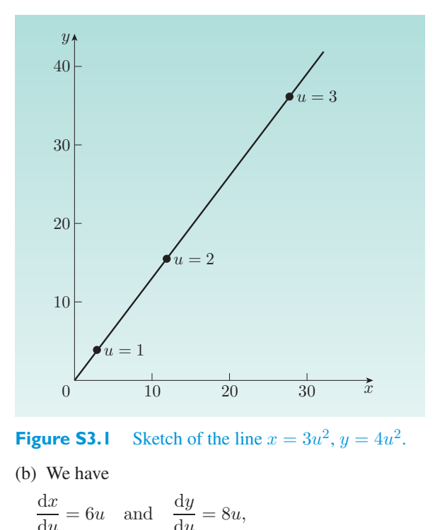
so所以
Exercise 3.2 Since r = R and \(\phi\) = u, we have d r = 0 and d \(\phi\) = d u, so练习 3.2 由于 r = R 且 \(\phi\) = u,我们有 d r = 0 且 d \(\phi\) = d u,因此
Exercise 3.3 (a) Like the cylinder, the cone can be formed by rolling up a练习 3.3 (a) 与圆柱体一样,圆锥体也可以通过卷起一个圆柱体来形成
region of the plane. Once again this won’t change the geometry; the circles and triangles will have the same properties as they have on the plane. So the cone has flat geometry.平面的区域。再次强调,这不会改变几何形状;圆形和三角形将具有与平面上相同的属性。所以圆锥体具有平坦的几何形状。
(b) In this case, distances for the bugs are shorter towards the edge of the disc, so the shortest distance from P to Q, as measured by the bugs, will appear to us to curve outwards. The angles of the triangle PQR add up to more than 180 ◦, as shown in Figure 3.12, so for this inverse hotplate the results are qualitatively similar to the geometry of the sphere, and the hotplate again has intrinsically curved geometry despite the lack of any extrinsic curvature.(b) 在这种情况下,虫子距离圆盘边缘的距离较短,因此虫子测量的从 P 到 Q 的最短距离在我们看来是向外弯曲的。三角形 PQR 的角度加起来超过 180°,如图 3.12 所示,因此对于这个反热板,结果在性质上与球体的几何形状相似,并且尽管缺乏任何外在曲率,但热板再次具有本质弯曲的几何形状。
Exercise 3.4 From Equation 3.10, we have练习 3.4 根据方程 3.10,我们有
Again there are only squared coordinate differentials, so \(g_{ij}\) = 0 for \(i\ne j\). We = \(R^2\) sin 2 \(x^1\), so can also see that g = \(R^2\) and g同样,只有平方坐标微分,因此对于 \(i\ne j\),\(g_{ij}\) = 0。我们 = \(R^2\) sin 2 \(x^1\),所以也可以看到 g = \(R^2\) 和 g
Exercise 3.5 In this case we only have squared coordinate differentials, so练习 3.5 在这种情况下,我们只有平方坐标微分,所以
g = 0 for \(i\ne j\). Also, g = 1, g = (\(x^1\)) 2, g = (\(x^1\)) 2 sin 2 \(x_{2}\), and therefore当 \(i\ne j\) 时,g = 0。另外,g = 1、g = (x 1) 2、g = (x 1) 2 sin 2 x 2,因此
Note that the final entry involves the coordinate \(x_{2}\), not x squared.请注意,最终条目涉及坐标 \(x_{2}\),而不是 x 平方。
Exercise 3.6 Defining \(x^1\) = r and \(x_{2}\) = \(\phi\), we have练习3.6 定义 \(x^1\) = r 和 \(x_{2}\) = \(\phi\),我们有
Exercise 3.7 (a) Since the line element is \(dl^2\) = (d \(x^1\)) 2 + (\((dx)^2\)) 2, we have练习 3.7 (a) 由于线元素为 \(dl^2\) = (d \(x^1\)) 2 + (\((dx)^2\)) 2,我们有
From Equation 3.23, the connection coefficients are defined by根据公式 3.23,联络系数定义为
and since ∂\(g_{ij}\)/∂x \(k = 0\) for all values of i, j, k, it follows that \(\Gamma^i{}_{jk}\) = 0 for all i, j, k.并且由于 ∂\(g_{ij}\)/∂x \(k = 0\) 对于所有 i、j、k 值,因此对于所有 i、j、k 来说 \(\Gamma^i{}_{jk}\) = 0。
Comment: This argument generalizes to any n-dimensional Euclidean space; consequently, when Cartesian coordinates are used, such spaces have vanishing connection coefficients.评论:这个论证推广到任何 n 维欧几里得空间;因此,当使用笛卡尔坐标时,此类空间的联络系数消失。
(b) From Exercise 3.4, the metric is(b) 从练习 3.4 中,度规为
and the dual metric is the inverse matrix对偶度规是逆矩阵
But in this case R = 1, so但在这种情况下 R = 1,所以
Since自从
there are six independent connection coefficients:有六个独立的联络系数:
However,然而,
while尽管
for all other values of i, j, k. Also, g il = 0 for \(i\ne l\), from which we can see that对于 i、j、k 的所有其他值。另外,对于 \(i\ne l\),g il = 0,由此我们可以看出
Consequently, the only non-zero values of the six independent connection coefficients listed above are因此,上面列出的六个独立联络系数中唯一的非零值是
and和
(The only other non-zero connection coefficient is Γ 2 21 = Γ 2 12.)(唯一的其他非零联络系数是 Г 2 21 = Г 2 12。)
Exercise 3.8 From Exercise 3.7(a), \(\Gamma^i{}_{jk}\) = 0 for all i, j, k in this metric, so练习 3.8 从练习 3.7(a) 中,对于该度规中的所有 i、j、k, \(\Gamma^i{}_{jk}\) = 0,因此
Equation 3.27 reduces to公式 3.27 简化为
giving the solutions x i = a \(\lambda\) + b for constants a, b. Writing this as x (\(\lambda\)) = aλ + b and y (\(\lambda\)) = cλ + d, we see that these equations parameterize the straight line through (b, d) with gradient c/a.给出常数 a、b 的解 x i = a \(\lambda\) + b。将其写为 x (\(\lambda\)) = aλ + b 和 y (\(\lambda\)) = cλ + d,我们看到这些方程以梯度 c/a 参数化通过 (b, d) 的直线。
Exercise 3.9 Using our usual coordinates for the surface of a sphere, \(x^1\) = \(\theta\),练习 3.9 使用我们通常的球体表面坐标,\(x^1\) = \(\theta\),
\(x_{2}\) = \(\phi\), and the results of Exercise 3.7(b) for the connection coefficients, Equation 3.27 becomes\(x_{2}\) = \(\phi\),练习 3.7(b) 的联络系数结果,公式 3.27 变为
and和
(a) The portion of a meridian A can be parameterized by so we have(a) 子午线 A 的部分可以通过以下方式参数化,因此我们有
Equation 3.69 becomes公式 3.69 变为
and Equation 3.70 becomes方程 3.70 变为
So A satisfies the geodesic equations and is a geodesic.因此 A 满足测地线方程并且是测地线。
Comment: This is what we would expect, because A is part of a great circle.评论:这正是我们所期望的,因为 A 是大圆的一部分。
(b) B can be parameterized by(b) B 可以通过以下方式参数化
So we have所以我们有
Equation 3.69 becomes 0 − 1 × 0 × 1 = 0, and Equation 3.70 becomes 0 + 2 × 0 × 1 × 0 = 0. So B satisfies the geodesic equations and is a geodesic.方程 3.69 变为 0 − 1 × 0 × 1 = 0,方程 3.70 变为 0 + 2 × 0 × 1 × 0 = 0。因此 B 满足测地线方程并且是测地线。
(c) C can be parameterized by(c) C 可以通过以下方式参数化
So we have所以我们有
Equation 3.69 becomes 0 − 2 × 2 × 1 = − 2 3 = 0, and Equation 3.70 becomes 0 + 2 × 1 × 0 × 1 = 0. So C is not a geodesic because it doesn’t satisfy both geodesic equations.方程 3.69 变为 0 − 2 × 2 × 1 = − 2 3 = 0,方程 3.70 变为 0 + 2 × 1 × 0 × 1 = 0。因此 C 不是测地线,因为它不满足两个测地线方程。
Exercise 3.10 (a) Since k is constant at every point on the curve and练习 3.10 (a) 由于 k 在曲线上的每个点都是常数,并且
k = 1/R, we havek = 1/R,我们有
= 5 cm. k 0.2 c\(\mathrm{m^{-1}}\)= 5 厘米。 k 0.2 厘米 - 1
So the best approximating circle at every point on the curve is a circle of radius 5 cm, and the curve itself is a circle of radius 5 cm.因此曲线上每一点的最佳近似圆是半径为 5 厘米的圆,并且曲线本身也是半径为 5 厘米的圆。
(b) Here again k will be constant, as the straight line has constant ‘curvature’. However big we draw the circle, a larger circle will approximate the straight line better, so the curvature of a straight line must be smaller than 1/R for all possible R. Hence k must be zero. In other words,(b) 这里 k 仍然是常数,因为直线具有常数“曲率”。无论我们画的圆有多大,较大的圆都会更好地逼近直线,因此对于所有可能的 R,直线的曲率必须小于 1/R。因此 k 必须为零。换句话说,
Exercise 3.11 The parabola can be parameterized by x (\(\lambda\)) = \(\lambda\) and y (\(\lambda\)) = \((\lambda)^2\)练习 3.11 抛物线可以通过 x (\(\lambda\)) = \(\lambda\) 和 y (\(\lambda\)) = \((\lambda)^2\) 进行参数化
. Consequently,。最后,
and for \(\lambda\) = 0 we have对于 \(\lambda\) = 0 我们有
So the curvature at \(\lambda\) = 0 is所以 \(\lambda\) = 0 处的曲率是
and the approximating circle has the radius近似圆的半径为
The centre of the circle is at x = 0, y = 0.5.圆心位于 x = 0、y = 0.5 处。
Exercise 3.12 The derivatives of x and y are given by练习 3.12 x 和 y 的导数由下式给出
so the curvature is given by所以曲率由下式给出
For the circle of radius R we have a = R and b = R, so对于半径为 R 的圆,我们有 a = R 和 b = R,所以
which is as expected.正如预期的那样。
Exercise 3.13 Interchanging the j, k indices in Equation 3.35, we get练习3.13 交换公式3.35中的j、k指数,我们得到
Swapping the first and second terms, and the third and fourth terms, leads to交换第一项和第二项以及第三项和第四项,导致
Comparison with Equation 3.35 shows that the expression on the right-hand side of this equation is − \(R^l{}_{ijk}\), hence proving that \(R^l{}_{ijk}\) = − \(R^l{}_{ikj}\).与式 3.35 比较可知,式右边的表达式为 − \(R^l{}_{ijk}\),从而证明 \(R^l{}_{ijk}\) = − \(R^l{}_{ikj}\)。
Exercise 3.14 From Exercise 3.7(a), all connection coefficients for this space练习 3.14 从练习 3.7(a) 中,该空间的所有联络系数
are zero, and hence from Equation 3.35, we have为零,因此根据公式 3.35,我们有
Since the connection coefficients also vanish for an n-dimensional space, it follows that the Riemann tensor is zero for such spaces.由于 n 维空间的联络系数也消失,因此黎曼张量对于此类空间为零。
Exercise 3.15 From Equation 3.35 and Exercise 3.7(b), we have练习 3.15 根据方程 3.35 和练习 3.7(b),我们有
But from Exercise 3.7(b),但根据练习 3.7(b),
so所以
Exercise 3.16 From the earlier in-text question, we know that K = a − 2, and练习 3.16 从前面的文本问题中,我们知道 K = a − 2,并且
from Exercise 3.15,从练习 3.15 中,
However, from Exercise 3.7(b),然而,根据练习 3.7(b),
so所以
Also, from Chapter 2 we know that lowering the first index on \(R^{1}\) 212 gives另外,从第 2 章我们知道,降低 \(R^1{}_{212}\) 上的第一个索引可以得到
However, \(g_{12}=0\), hence然而,\(g_{12}=0\),因此
which is the same as K.与 K 相同。
Exercise 3.17 (a) Just as in Exercise 3.7(a), the connection coefficients are练习 3.17 (a) 正如练习 3.7(a) 中一样,联络系数为
zero since the metric is constant.零,因为度规是恒定的。
(b) Since the connection coefficients for a Minkowski spacetime are zero, as shown in part (a), and each term in the Riemann tensor defined by Equation 3.35 involves at least one connection coefficient, it follows that all components of the Riemann tensor are zero.(b) 由于闵可夫斯基时空的联络系数为零,如 (a) 部分所示,并且方程 3.35 定义的黎曼张量中的每一项至少涉及一个联络系数,因此黎曼张量的所有分量都为零。
Exercise 3.18 (a) The metric is练习 3.18 (a) 度规为
and the dual metric is对偶度规是
As in Exercise 3.7(b), there are only six independent connection coefficients:如练习 3.7(b) 所示,只有六个独立的联络系数:
Moreover,而且,
11 = − 2 f f ˙, where f ˙ ≡11 = − 2 f f ˙, 其中 f ˙ ≡
and和
for all other values of i, j, k. Also, g il = 0 for \(i\ne l\), from which we can see that对于 i、j、k 的所有其他值。另外,对于 \(i\ne l\),g il = 0,由此我们可以看出
Consequently, the only non-zero values of the six independent connection coefficients listed above are因此,上面列出的六个独立联络系数中唯一的非零值是
and和
The only other non-zero connection coefficient is Γ 1 10 = Γ 1 01.唯一的其他非零联络系数是 Г 1 10 = Г 1 01。
(b) As in Exercise 3.15,(b) 如练习 3.15 所示,
Since Γ 0 = Γ 0 = Γ 0 = Γ 1 = Γ 1 = 0, we have由于 Г 0 = Г 0 = Г 0 = Г 1 = Г 1 = 0,我们有
Exercise 4.1 (a) Suppose that the separation is l and the distance from the练习 4.1 (a) 假设间隔为 l,距
centre of the Earth is R, as shown in Figure S4.1.地球中心为R,如图S4.1所示。
Then the magnitude of the horizontal acceleration of each object is g sin \(\theta\) ≈ gθ, so the total (relative) acceleration is g 2 \(\theta\). However, 2 \(\theta\) = l/R, so the magnitude of the total acceleration, a, is given by那么每个物体的水平加速度大小为 g sin \(\theta\) ≈ gθ,因此总(相对)加速度为 g 2 \(\theta\)。然而,2 \(\theta\) = l/R,因此总加速度 a 的大小由下式给出
\(\mathrm{m\,s^{-2}}\) = \(3.08\times10^{-6}\) \(\mathrm{m\,s^{-2}}\).\(\mathrm{m\,s^{-2}}\) = \(3.08\times10^{-6}\) \(\mathrm{m\,s^{-2}}\)。
(b) Suppose that one object is a distance l vertically above the other object. Since Newtonian gravity is an inverse square law, the magnitudes of acceleration at R and R + l are related by(b) 假设一个物体位于另一个物体上方垂直距离 l 处。由于牛顿引力是平方反比定律,因此 R 和 R + l 处的加速度大小与下式相关:
Hence \(\Delta g\), the difference between the magnitudes of acceleration at R and R + l, is given by因此,R 和 R + l 处的加速度大小之差 \(\Delta g\) 由下式给出
\(\mathrm{m\,s^{-2}}\) = \(6.15\times10^{-6}\) \(\mathrm{m\,s^{-2}}\).\(\mathrm{m\,s^{-2}}\) = \(6.15\times10^{-6}\) \(\mathrm{m\,s^{-2}}\)。
Exercise 4.2练习4.2
(a) As indicated by Figure S4.2, the coordinates are related by x = r cos \(\theta\), y = r sin \(\theta\).(a) 如图 S4.2 所示,坐标关系为 x = r cos \(\theta\),y = r sin \(\theta\)。
Setting (\(x'_{1}\), \(x'_{2}\)) = (x, y) and (\(x^1\), \(x_{2}\)) = (r, \(\theta\)), we have设置 (\(x'_{1}\), \(x'_{2}\)) = (x, y) 且 (\(x^1\), \(x_{2}\)) = (r, \(\theta\)),我们有
and和
In this case, the general tensor transformation law reduces to在这种情况下,一般张量变换定律简化为
A \(\nu\), and \(A'_{2}\) =\(\nu\),\(A'_{2}\) =
This means that \(A'\) \(\mu\) and A \(\mu\) must be related by这意味着 \(A'\) \(\mu\) 和 A \(\mu\) 必须通过以下方式关联
and \(A'_{2}\) = sin \(\theta\) A 1 + r cos \(\theta\) A 2.\(A'_{2}\) = sin \(\theta\) A 1 + r cos \(\theta\) A 2。
(b) In the case of the infinitesimal displacement, this general transformation rule implies that(b) 在无穷小的位移的情况下,这个一般变换规则意味着
d x = cos \(\theta\) d r − r sin \(\theta\) d \(\theta\), and d y = sin \(\theta\) d r + r cos \(\theta\) d \(\theta\).d x = cos \(\theta\) d r − r sin \(\theta\) d \(\theta\),并且 d y = sin \(\theta\) d r + r cos \(\theta\) d \(\theta\)。
But this is exactly the relationship between these different sets of coordinates given by the chain rule, so the infinitesimal displacement does transform as a contravariant rank 1 tensor.但这正是链式法则给出的这些不同坐标集之间的关系,因此无穷小的位移确实变换为逆变 1 阶张量。
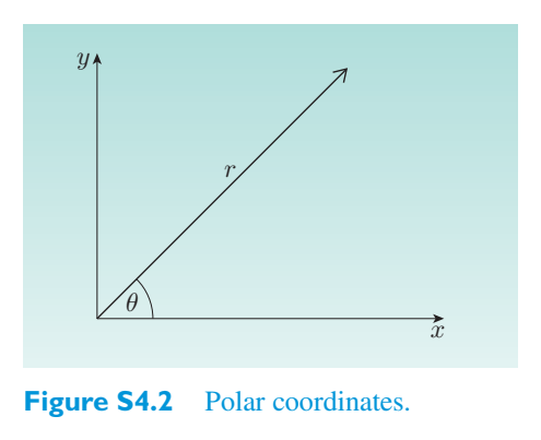
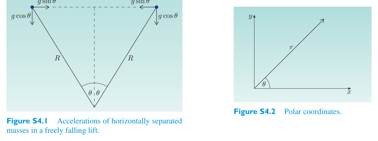
Exercise 4.3 We know that练习4.3 我们知道
Multiplying by g \(\nu\)\(\mu\) and summing over \(\mu\), we have乘以 g \(\nu\)\(\mu\) 并对 \(\mu\) 求和,我们有
Reversing the order in which we do the summation on the right-hand side of this equation enables us to write it as颠倒我们在方程右侧求和的顺序,我们可以将其写为
However,然而,
Since δ \(\nu\) = 1 when \(\nu\) = \(\alpha\) and δ \(\nu\) = 0 when \(\nu\) 3 = \(\alpha\), we have由于当 \(\nu\) = \(\alpha\) 时 δ \(\nu\) = 1,当 \(\nu\) 3 = \(\alpha\) 时 δ \(\nu\) = 0,我们有
Exercise 4.4 (a) There are two reasons. The \(\mu\) index is up on A \(\mu\) but down练习 4.4 (a) 有两个原因。 \(\mu\) 指数在 A \(\mu\) 上上升,但在下降
on B \(\mu\). The K term has no \(\mu\) index.在 B \(\mu\) 上。 K 项没有 \(\mu\) 索引。
(b) The \(\nu\) index cannot be up on both Y \(\mu\)\(\nu\) and Z \(\nu\); it must be up on one term and down on the other.(b) \(\nu\) 指数不能在 Y \(\mu\)\(\nu\) 和 Z \(\nu\) 上同时上涨;它必须在一项上上升,而在另一项上下降。
(c) There cannot be three instances of the \(\nu\) index on the right-hand side of this equation.(c) 该等式右侧不能有 \(\nu\) 索引的三个实例。
Exercise 4.5 Being a scalar, this quantity has no contravariant or covariant练习 4.5 作为标量,该量没有逆变或协变
indices. So in this particular case, covariant differentiation simply gives指数。所以在这种特殊情况下,协变微分简单地给出
Exercise 4.6 We know that练习4.6 我们知道
and和
Since \(U^0=c\) in the instantaneous rest frame, we have \(T^{00}=\rho c^2\). Also, \(T^{0i}=0\) since \(\eta^{0i}=0\) and \(U^i=0\) in this frame. Likewise,由于瞬时静止坐标系中的 \(U^0=c\),我们有 \(T^{00}=\rho c^2\)。此外,\(T^{0i}=0\) 自从该帧中的 \(\eta^{0i}=0\) 和 \(U^i=0\) 开始。同样地,
Finally, for \(i\ne j\),最后,对于 \(i\ne j\),
since \(\eta^{ij}=0\) for \(i\ne j\) and \(U^i=0\) in the instantaneous rest frame.因为在瞬时静止坐标系中,对于 \(i\ne j\) 有 \(\eta^{ij}=0\),并且 \(U^i=0\)。
Exercise 4.7 Multiplying Equation 4.34 by \(g_{\mu\nu}\) and summing over both练习 4.7 将方程 4.34 乘以 \(g_{\mu\nu}\) 并对两者求和
indices, we obtain指数,我们得到
Now using the fact that现在利用这样的事实
this becomes这变成
Hence R = κT, which we can substitute in Equation 4.34 to obtain Equation 4.35:因此,R = κT,我们可以将其代入公式 4.34 以获得公式 4.35:
so所以
Exercise 5.1 From the definition of the Einstein tensor,练习 5.1 根据爱因斯坦张量的定义,
and we have and我们有并且
So所以
as required.根据需要。
Exercise 5.2 (a) The only place where the coordinate \(\phi\) appears in the练习 5.2 (a) 坐标 \(\phi\) 出现在
Schwarzschild line element is in the term \(r^2\) \(\sin^2 \theta\) (d \(\phi\)) 2. But since \(\phi'\) = \(\phi\) + \(\phi\), the difference in the \(\phi\) -coordinates of any two events will be equal to the difference in the \(\phi'\)-coordinates of those events, and in the limit, for infinitesimally separated events, d \(\phi'\) = d(\(\phi\) + \(\phi\)) = d \(\phi\). So the Schwarzschild line element is unaffected by the change of coordinates apart from the replacement of \(\phi\) by \(\phi'\). This establishes the form-invariance of the metric under the change of coordinates.史瓦西线元的术语为 \(r^2\) \(\sin^2 \theta\) (d \(\phi\)) 2。但由于 \(\phi'\) = \(\phi\) + \(\phi\),任何两个事件的 \(\phi\) 坐标之差将等于这些事件的 \(\phi'\) 坐标之差,并且在极限情况下,对于无限小的分离事件,d \(\phi'\) = d(\(\phi\) + \(\phi\)) = d \(\phi\)。因此,除了将 \(\phi\) 替换为 \(\phi'\) 之外,史瓦西线元不受坐标变化的影响。这建立了坐标变化下度规的形式不变性。
(b) In a system of spherical coordinates, a given value of the coordinate \(\phi\) corresponds to a meridian of the kind shown in Figure S5.1.(b) 在球坐标系中,给定的坐标 \(\phi\) 值对应于图 S5.1 所示的子午线。
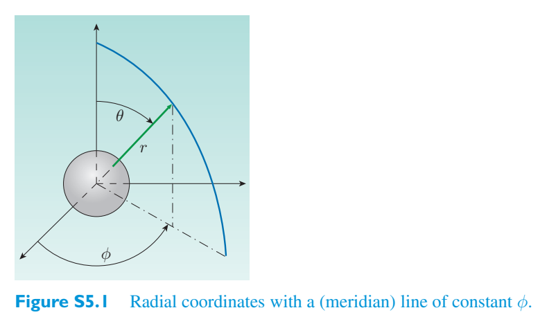
Exercise 5.3 We require练习 5.3 我们要求
With d r = d \(\theta\) = d \(\phi\) = 0 the metric reduces to当 d r = d \(\theta\) = d \(\phi\) = 0 时,度规减少为
so所以
Rearranging gives重新排列给出
= \(1.5\times10^{11}\) metres.= \(1.5\times10^{11}\) 米。
We have not yet found the relationship between the Schwarzschild coordinate r and physical (proper) distance — that is the subject of the next section. Nonetheless it is interesting to note that a proper distance of \(1.5\times10^{11}\) metres is about the distance from the Earth to the Sun.我们还没有找到史瓦西坐标 r 和物理(适当)距离之间的关系——这是下一节的主题。尽管如此,有趣的是,\(1.5\times10^{11}\) 米的固有距离大约是地球到太阳的距离。
Exercise 5.4 The proper distance d \(\sigma\) between two neighbouring events that练习 5.4 两个相邻事件之间的固有距离 d \(\sigma\)
happen at the same time (d t = 0) is given by the metric via the relationship (d s) 2 = − (d \(\sigma\)) 2. Thus同时发生 (d t = 0) 由度规通过关系 (d s) 2 = − (d \(\sigma\)) 2 给出。因此
For the circumference at a given r -coordinate in the \(\theta\) = \(\pi\)/2 plane, d r = d \(\theta\) = 0, hence对于 \(\theta\) = \(\pi\)/2 平面中给定 r 坐标处的周长,d r = d \(\theta\) = 0,因此
So所以
and therefore因此
as required.根据需要。
Exercise 5.5 It follows from the general equation for an affinely parameterized练习 5.5 由仿射参数化的一般方程得出
geodesic that测地线
Since the only non-zero connection coefficients with a raised index 0 are Γ 0 01 = Γ 0 10, the sum may be expanded to give由于索引为 0 的唯一非零联络系数为 Γ 0 01 = Γ 0 10,因此总和可展开为
Identifying \(x^0\) = ct, \(x^1\) = r and Γ 0 =! GM B, we see that识别 \(x^0\) = ct、\(x^1\) = r 和 Γ 0 =! GM B,我们看到了
as required.根据需要。
Exercise 5.6 For circular motion at a given r -coordinate in the equatorial练习 5.6 对于赤道上给定 r 坐标的圆周运动
plane, u is constant, so平面,u 是常数,所以
= 0 and also= 0 并且还有
(a) It follows from the orbital shape equation (Equation 5.36) that for a circular orbit with J 2/\(m^{2}\) = 12 \(G^{2}\) M 2/\(c^2\),(a) 由轨道形状方程(方程 5.36)得出,对于 J 2/\(m^{2}\) = 12 \(G^{2}\) M 2/\(c^2\) 的圆形轨道,
i.e.IE。
Solving this quadratic equation in u gives u = \(c^2\)/6 GM, so r = 6 GM/\(c^2\) is the minimum radius of a stable circular orbit.求解 u 中的这个二次方程得到 u = \(c^2\)/6 GM,因此 r = 6 GM/\(c^2\) 是稳定圆形轨道的最小半径。
(b) The corresponding value of E may be determined from the radial motion equation (Equation 5.32), remembering that d r/d \(\tau\) = 0:(b) E 的对应值可以根据径向运动方程(方程 5.32)确定,记住 d r/d \(\tau\) = 0:
So所以
Simplifying this, we have简化这个,我们有
or或者
which can be rearranged to give E = 8 \(mc^2\)/3.可以重新排列得到 E = 8 \(mc^2\)/3。
Exercise 6.1 (a) For the Sun, \(R_S\) = 3 km. So for a black hole with three times练习 6.1 (a) 对于太阳,RS = 3 km。所以对于一个有三倍的黑洞
the Sun’s mass, the Schwarzschild radius is 9 km. Substituting this value into Equation 6.10, we find that the proper time required for the fall is just太阳的质量,史瓦西半径是9公里。将该值代入公式 6.10,我们发现下降所需的固有时间为
\(\tau\) = \(6\times10^{3}\)/(\(3\times10^{8}\)) s = \(2\times10^{-5}\) s.\(\tau\) = \(6\times10^{3}\)/(\(3\times10^{8}\)) s = \(2\times10^{-5}\) s。
(b) For a \(10^9M_\odot\) galactic-centre black hole, the Schwarzschild radius and the in-fall time are both greater by a factor of \(10^9/3\). A calculation similar to that in part (a) therefore gives a free fall time of 6700 s, or about 112 minutes. (Note that these results apply to a body that starts its fall from far away, not from the horizon.)(b) 对于 \(10^9M_\odot\) 银心黑洞,史瓦西半径和坠落时间都大 \(10^9/3\) 倍。因此,与 (a) 部分类似的计算得出的自由落体时间为 6700 秒,即大约 112 分钟。 (请注意,这些结果适用于从远处开始下落的物体,而不是从地平线开始下落的物体。)
Exercise 6.2 According to Equation 6.12, for events on the world-line of a练习 6.2 根据方程 6.12,对于某个世界线上的事件
radially travelling photon,径向行进的光子,
For a stationary local observer, i.e. an observer at rest at r, we saw in Chapter 5 that intervals of proper time are related to intervals of coordinate time by \(d\tau=dt(1-R_S/r)^{1/2}\), while intervals of proper distance are related to intervals of coordinate distance by \(d\sigma=dr(1-R_S/r)^{-1/2}\). It follows that the speed of light as measured by a local observer, irrespective of their location, will always be对于静止的本地观察者,即在 r 处静止的观察者,我们在第 5 章中看到,本征时间间隔与坐标时间间隔 \(d\tau=dt(1-R_S/r)^{1/2}\) 相关,而固有距离间隔与坐标距离间隔 \(d\sigma=dr(1-R_S/r)^{-1/2}\) 相关。由此可见,由当地观察者测量的光速,无论其位置如何,始终是
So, in the case that the intervals being referred to are those between events on the world-line of a radially travelling photon, we see that the locally observed speed of the photon is因此,在所提到的间隔是径向行进光子的世界线上的事件之间的间隔的情况下,我们看到局部观察到的光子速度是
Exercise 6.3 According to the reciprocal of Equation 6.17, for events on the练习 6.3 根据方程 6.17 的倒数,对于
world-line of a freely falling body,自由落体的世界线,
We already know from the previous exercise that for a stationary local observer,从之前的练习中我们已经知道,对于静止的本地观察者,
So, in the case of a freely falling body, the measured inward radial velocity will be因此,在自由落体的情况下,测得的向内径向速度将为
In the limit as r → \(R_S\), the locally observed speed is given by | d \(\sigma\)/d \(\tau\) | → c.在 r → \(R_S\) 的极限中,局部观察到的速度由下式给出: d \(\sigma\)/d \(\tau\) | → c.
Exercise 6.4 Initially, the fall would look fairly normal with the astronaut练习 6.4 最初,宇航员的跌倒看起来相当正常
apparently getting smaller and picking up speed as the distance from the observer increased. At first the frequency of the astronaut’s waves would also look normal, though detailed measurements would reveal a small decrease due to the Doppler effect. As the distance increased, the astronaut’s speed of fall would continue to increase and the frequency of waving would decrease. This would be accompanied by a similar change in the frequency of light received from the falling astronaut, so the astronaut would appear to become redder as well as more distant. As the astronaut approached the event horizon, the effect of spacetime distortion would become dominant. The astronaut’s rate of fall would be seen to decrease, but the image would become very red and would rapidly dim, causing the departing astronaut to fade away.随着与观察者的距离增加,显然变得越来越小并且速度加快。起初,宇航员的电波频率看起来也很正常,但详细的测量结果显示,由于多普勒效应,频率略有下降。随着距离的增加,宇航员下落的速度会不断增加,挥手的频率会减少。这会伴随着从坠落的宇航员接收到的光频率的类似变化,因此宇航员看起来会变得更红,也更远。当宇航员接近视界时,时空扭曲的影响将变得占主导地位。宇航员的下落速度会降低,但图像会变得非常红并迅速变暗,导致离开的宇航员逐渐消失。
Though something along these lines is the expected answer, there is another effect to take into account, that depends on the mass of the black hole. This is a consequence of tidal forces and will be discussed in the next section.虽然沿着这些思路是预期的答案,但还有另一个影响需要考虑,这取决于黑洞的质量。这是潮汐力的结果,将在下一节中讨论。
Exercise 6.5 The increasing narrowness and gradual tipping of the lightcones练习 6.5 光锥逐渐变窄和逐渐倾斜
as they approach the event horizon indicates the difficulty of outward escape for photons and, by implication, for any particles that travel slower than light. This effect reaches a critical stage at the event horizon, where the outgoing edge of the lightcone becomes vertical, indicating that even photons emitted in the outward direction are unable to make progress in that direction. A diagrammatic study of lightcones alone is unable to prove the impossibility of escape from within the event horizon, but the progressive narrowing and tipping of lightcones in that region is at least suggestive of the impossibility of escape, and it is indeed a fact that all affinely parameterized geodesics that enter the event horizon of a non-rotating black hole reach the central singularity at some finite value of the affine parameter.当它们接近事件视界时,表明光子向外逃逸的难度,暗示任何比光慢的粒子向外逃逸的难度。这种效应在事件视界达到关键阶段,光锥的出射边缘变得垂直,这表明即使向外发射的光子也无法在该方向上前进。仅对光锥进行图解研究无法证明从事件视界内逃逸的不可能性,但该区域中光锥的逐渐缩小和倾斜至少暗示了逃逸的不可能性,而且事实上,进入非旋转黑洞事件视界的所有仿射参数化测地线都在仿射参数的某个有限值处到达中心奇点。
Exercise 6.6 The time-like geodesic for the Schwarzschild case has already练习 6.6 史瓦西案例的类时间测地线已经
been given in Figure 6.11. The nature of the lightcones is also represented in that figure, so the expected answer is shown in Figure S6.1a. In the case of Eddington–Finkelstein coordinates, Figure 6.13 plays a similar role, suggesting (rather than showing) the form of the time-like geodesic and indicating the form of the lightcones. The expected answer is shown in Figure S6.1b.已在图 6.11 中给出。该图中也表示了光锥的性质,因此预期的答案如图 S6.1a 所示。在爱丁顿-芬克尔斯坦坐标的情况下,图 6.13 起着类似的作用,暗示(而不是显示)类时间测地线的形式并指示光锥的形式。预期答案如图 S6.1b 所示。
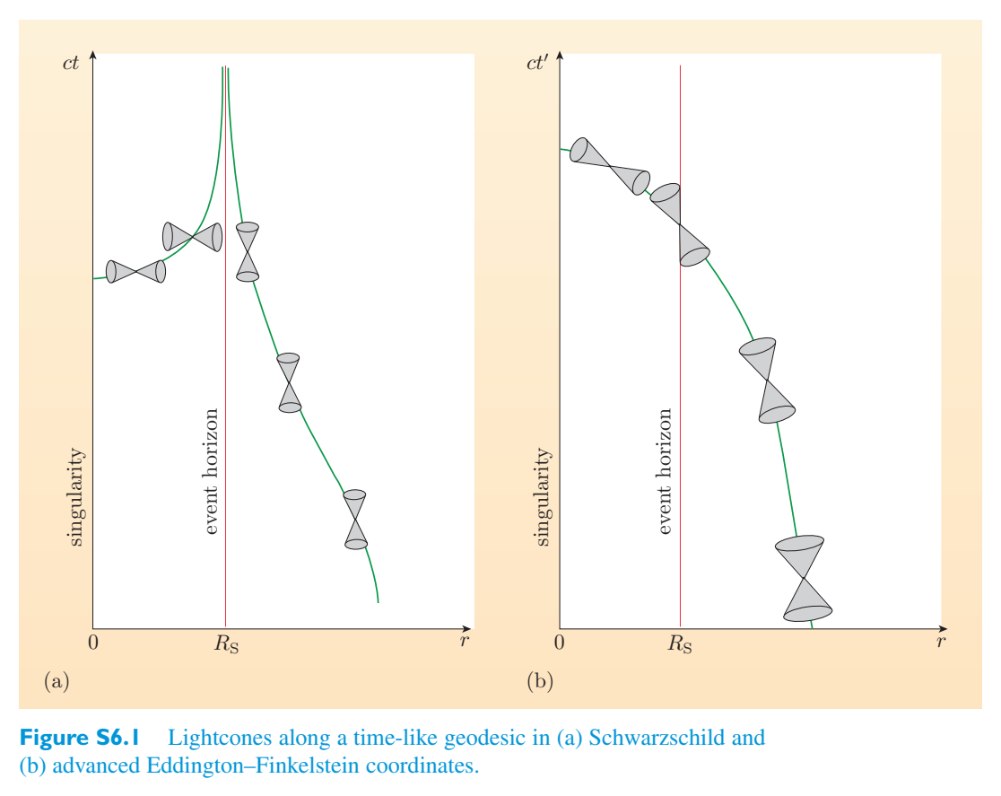
Exercise 6.7 (a) When \(J=Gm^2/c\), we have \(a=J/(Mc)=GM/c^2=R_S/2\)练习 6.7 (a) 当 \(J=Gm^2/c\) 时,我们有 \(a=J/(Mc)=GM/c^2=R_S/2\)
. Inserting this into Equations 6.32 and 6.33, the second term vanishes and we find r = R/2.。将其代入方程 6.32 和 6.33,第二项消失,我们发现 r = R/2。
(b) When J = 0, we have a = 0 and we obtain r = R, r = 0.(b) 当 J = 0 时,a = 0,并得到 r = R,r = 0。
In both cases (a) and (b), there is only one event horizon as the inner horizon vanishes.在 (a) 和 (b) 两种情况中,当内视界消失时,只有一个事件视界。
Exercise 6.8 (a) The path indicated by the dashed line in Figure 6.20 shows练习 6.8 (a) 图 6.20 中虚线所示的路径
no change in angle as it approaches the static limit. Space outside the static limit is also dragged around, even though rotation is no longer compulsory. However, a particle in free fall must be affected by this dragging, and so a particle in free fall could not fall in on the dashed line. The path of free fall would have to curve in the direction of rotation of the black hole.当接近静态极限时,角度没有变化。即使不再强制旋转,静态限制之外的空间也会被拖动。然而,自由落体中的粒子一定会受到这种拖动的影响,因此自由落体中的粒子不能落在虚线上。自由落体的路径必须沿着黑洞旋转的方向弯曲。
(b) It is possible to follow the dashed path, but the spacecraft would have to exert thrust to counteract the effects of the spacetime curvature of the rotating black hole that make the paths of free fall have a decreasing angular coordinate.(b) 可以沿着虚线路径行走,但航天器必须施加推力来抵消旋转黑洞的时空曲率的影响,这种影响使自由落体的路径具有递减的角坐标。
(c) The dotted path represents an impossible trip for the spacecraft. Inside the ergosphere, no amount of thrust in the anticlockwise direction can make the spacecraft maintain a constant angular coordinate while decreasing the radial coordinate.(c) 虚线路径代表航天器不可能的旅行。在能层内,无论逆时针方向多大的推力都无法使航天器在减小径向坐标的同时保持恒定的角坐标。
Exercise 6.9 The discovery of a mini black hole would imply (contrary to most练习 6.9 迷你黑洞的发现意味着(与大多数人的观点相反)
expectations) that conditions during the Big Bang were such as to lead to the production of mini black holes. This would be an important development for cosmology.预期)大爆炸期间的条件会导致迷你黑洞的产生。这将是宇宙学的一个重要发展。
Such a discovery would also open up the possibility of confirming the existence of Hawking radiation, thus giving some experimental support to attempts to weld together quantum theory and general relativity, such as string theory.这样的发现也将开启确认霍金辐射存在的可能性,从而为将量子理论和广义相对论(例如弦理论)结合在一起的尝试提供一些实验支持。
Exercise 7.1 We first need to decide how many days make up a century. This is练习7.1 我们首先需要确定一个世纪有多少天。这是
not entirely straightforward because leap years don’t simply occur every 4 years in the Gregorian calendar. However, it is the Julian year that is used in astronomy and this is defined so that one year is precisely 365.25 days. Consequently we have 36 525 days per century, which we denote by d. If we use T to denote the period of the orbit in (Julian) days, then the number of orbits per century is d/T. Equation 7.1 gives the angle in radians, but it is more usual to express the observations in seconds of arc so we need to use the fact that \(\pi\) radians equals 180 × 3600 seconds of arc. Putting all this together, we find that the general relativistic contribution to the mean rate of precession of the perihelion in seconds of arc per century is given by这并不完全简单,因为闰年并不是简单地在公历中每 4 年出现一次。然而,天文学中使用的是儒略年,并且这一年的定义是一年正好是 365.25 天。因此,每个世纪有 36 525 天,用 d 表示。如果我们用 T 来表示以(儒略)天为单位的轨道周期,则每世纪的轨道数量为 d/T。方程 7.1 给出了以弧度为单位的角度,但更常见的是以弧秒来表示观测值,因此我们需要使用 \(\pi\) 弧度等于 180 × 3600 弧秒这一事实。将所有这些放在一起,我们发现广义相对论对近日点平均进动率(以每世纪弧秒为单位)的贡献为
× 3 888 000 seconds of arc seconds of arc =× 3 888 000 弧秒弧秒 =
seconds of arc per century每世纪弧秒
Exercise 7.2 For rays just grazing the Sun, b is the radius of the Sun, which is练习7.2 对于刚刚掠过太阳的光线,b 是太阳的半径,即
R = \(6.96\times10^{8}\) m, and M is M = \(1.989\times10^{30}\) kg. Hence the deflection in seconds of arc is given byR = \(6.96\times10^{8}\) m,M 为 M = \(1.989\times10^{30}\) kg。因此,以弧秒为单位的偏转由下式给出
seconds of arc = seconds of arc弧秒 = 弧秒
Exercise 7.3 (a) Let R ⊕ = 6371.0 km be the mean radius of the Earth,练习 7.3 (a) 令 R ⊕ = 6371.0 km 为地球的平均半径,
M = \(5.9736\times10^{24}\) kg be the mass of the Earth, and h = 20 200 km be the height of the satellite above the Earth. From Equation 5.14, the coordinate time interval at R ⊕ and the coordinate time interval at R ⊕ + h are related byM = \(5.9736\times10^{24}\) kg 为地球质量,h = 20 200 km 为卫星距地球的高度。根据公式 5.14,R ⊕ 处的坐标时间间隔和 R ⊕ + h 处的坐标时间间隔的关系为:
Since the time dilation is small, we can use the first few terms of a Taylor expansion to evaluate this. Putting 2 M G/\(c^2\) (R + h) = x and 2 M G/\(c^2\) R = y, the right-hand side above becomes (1 − x) − 1/2 × (1 − y) 1/2. By a Taylor expansion, this is approximately (1 + x)(1 − y) ≈ 1 + x − y. So we have由于时间膨胀很小,我们可以使用泰勒展开式的前几项来评估这一点。将 2 MG/\(c^2\) (R + h) = x 和 2 MG/\(c^2\) R = y 代入,上面的右侧变为 (1 − x) − 1/2 × (1 − y) 1/2。通过泰勒展开式,这大约为 (1 + x)(1 − y) ≈ 1 + x − y。所以我们有
The discrepancy over 24 hours is given by24 小时内的差异由下式给出
× 24 × 3600 s× 24 × 3600 秒
= − 45.7 \(\mu\) s.= − 45.7 \(\mu\) 秒。
The negative sign indicates that the effect of general relativity is that the satellite clock runs more rapidly than a ground-based one.负号表明广义相对论的影响是卫星时钟比地面时钟运行得更快。
(b) Special relativity relates a time interval \(\Delta t\) for a clock moving at speed v with the time interval Δ \(t_0\) for one at rest by(b) 狭义相对论将时钟以速度 v 运动的时间间隔 \(\Delta t\) 与静止时钟的时间间隔 Δ \(t_0\) 联系起来:
For a satellite orbiting the Earth at a distance h from the Earth’s surface, its speed is given by对于距地球表面距离为 h 的绕地球运行的卫星,其速度由下式给出
and hence因此
Hence the discrepancy over 24 hours between satellite- and ground-based clocks is因此,卫星时钟和地面时钟之间 24 小时的差异为
× 24 × 3600 s× 24 × 3600 秒
= 7.2 \(\mu\) s.= 7.2 \(\mu\) 秒。
The positive result indicates that the effect of special relativity is that the satellite clock runs slower than a ground-based one.这一积极的结果表明,狭义相对论的效应是卫星时钟的运行速度比地面时钟慢。
(c) The total effect of the results obtained in parts (a) and (b) is a discrepancy between ground-based and satellite-based clocks of (− 45.7 + 7.2) = − 38.5 \(\mu\) s per day. Since the basis of the GPS is the accurate timing of radio pulses, over 24 hours this could lead to an error in distance of up to(c) (a) 和 (b) 部分获得的结果的总体影响是地面时钟和卫星时钟之间的差异为每天 (− 45.7 + 7.2) = − 38.5 \(\mu\) 秒。由于 GPS 的基础是无线电脉冲的精确定时,因此超过 24 小时可能会导致距离误差高达
c (\(\Delta t\) − \(\Delta t\)) = \(2.998\times10^{8}\) × \(38.5\times10^{-6}\) m = 11.5 km.c (\(\Delta t\) − \(\Delta t\)) = \(2.998\times10^{8}\) × \(38.5\times10^{-6}\) m = 11.5 公里。
Exercise 7.4 We can approximate the radius of the satellite’s orbit by the练习7.4 我们可以通过以下公式来近似卫星轨道的半径
Earth’s radius. Hence the period of the orbit, T, is given by地球的半径。因此,轨道周期 T 由下式给出
Since自从
Equation 7.13 can be approximated by方程 7.13 可以近似为
After a time Y, the number of orbits is Y/T and the total precession is given by经过 Y 时间后,轨道数为 Y/T,总进动由下式给出
total T总T
Converting from radians to seconds of arc, we find that the total precession angle for one year is从弧度转换为弧秒,我们发现一年的总进动角为
total全部的
Exercise 7.5 We have previously carried out a similar calculation for low练习7.5 我们之前已经对低值进行了类似的计算
Earth orbit, the only difference here being that the radius of the orbit is now R = (\(6.371\times10^{6}\) m) + (\(642\times10^{3}\) m) instead of \(6.371\times10^{6}\) m. Consequently, the expected precession is地球轨道,唯一的区别是轨道半径现在是 R = (\(6.371\times10^{6}\) m) + (\(642\times10^{3}\) m) 而不是 \(6.371\times10^{6}\) m。因此,预期进动为
Exercise 7.6 When considering light rays travelling from a distant source to a练习 7.6 当考虑光线从远处的光源传播到另一处的光源时
detector, it is not just one ray that travels from the source to the detector, but a cone of rays. Gravitational lensing effectively increases the size of the cone of rays that reach the detector. The light is not concentrated in the same way as in Figure 7.15, but it is concentrated.探测器,从光源传播到探测器的不仅仅是一条射线,而是一束射线。引力透镜有效地增加了到达探测器的光线锥体的尺寸。光线不像图 7.15 那样集中,但它是集中的。
Exercise 8.1 (i) On size scales significantly greater than 100 Mly, the练习 8.1 (i) 在尺寸尺度显着大于 100 Mly 时,
large-scale structure of voids and superclusters (i.e. clusters of clusters of galaxies) does indeed appear to be homogeneous and isotropic.空洞和超星系团(即星系团簇)的大尺度结构确实看起来是均匀且各向同性的。
(ii) After removing distortions due to local motions, the mean intensity of the cosmic microwave background radiation differs by less than one part in ten thousand in different directions. This too is evidence of isotropy and homogeneity.(ii) 消除局部运动引起的畸变后,宇宙微波背景辐射的平均强度在不同方向上的差异小于万分之一。这也是各向同性和同质性的证据。
(iii) The uniformity of the motion of galaxies on large scales, known as the Hubble flow, is a third piece of evidence in favour of a homogeneous and isotropic Universe.(iii) 大尺度上星系运动的均匀性,即哈勃流,是支持均匀且各向同性宇宙的第三个证据。
Exercise 8.2 Geodesics are found using the geodesic equation. The first step is练习 8.2 使用测地线方程求测地线。第一步是
to identify the covariant metric coefficients of the relevant space-like hypersurface (only \(g_{11}\), \(g_{22}\) and \(g_{33}\) will be non-zero). The contravariant form of the metric coefficients follows immediately from the requirement that \([g^{ij}]\) is the matrix inverse of \([g_{ij}]\). The covariant and contravariant components can then be used to determine the connection coefficients \(\Gamma^i{}_{jk}\). Once the connection coefficients for the hypersurface have been determined, the spatial geodesics may be found by solving the geodesic equation for the hypersurface. At that stage it would be sufficient to demonstrate that a parameterized path of the form \(r=r(\lambda)\), \(\theta=\mathrm{constant}\), \(\phi=\mathrm{constant}\) satisfies the geodesic equation for the hypersurface.识别相关类空超曲面的协变度规系数(只有 \(g_{11}\)、\(g_{22}\) 和 \(g_{33}\) 非零)。度规系数的逆变形式可由 \([g^{ij}]\) 是 \([g_{ij}]\) 的矩阵逆这一要求直接得到。随后可用协变和逆变分量确定联络系数 \(\Gamma^i{}_{jk}\)。确定超曲面的联络系数后,可以通过求解该超曲面的测地线方程找到空间测地线。在这一步,只需证明形如 \(r=r(\lambda)\)、\(\theta=\mathrm{constant}\)、\(\phi=\mathrm{constant}\) 的参数化路径确实满足该超曲面的测地线方程即可。
Exercise 8.3 The Minkowski metric differs in that it does not feature the scale练习8.3 闵可夫斯基度规的不同之处在于它不具有尺度
factor \(R(t)\). It is true that \(k = 0\) for both cases, and this means that space is flat. But the presence of the scale factor in the Robertson–Walker metric allows spacetime to be non-flat.因子 \(R(t)\)。确实,这两种情况都是 \(k = 0\),这意味着空间是平坦的。但罗伯逊-沃克度规中尺度因子的存在使得时空变得不平坦。
Exercise 8.4 We start with the energy equation练习8.4 我们从能量方程开始
and differentiate it with respect to time t. We use the product rule on the left-hand side and obtain并对时间 t 求导。我们使用左侧的乘积规则并得到
We then use the chain rule to replace d with d R d, which gives然后我们使用链式法则将 d 替换为 d R d,这给出
Then carrying out the various differentiations with respect to R, we get然后对R进行各种微分,我们得到
We then substitute back in for 1 d \(R^2\) in the first term on the left-hand side, using the energy equation again, to get然后,我们再次使用能量方程,将左侧第一项中的 1 d \(R^2\) 代入,得到
We now substitute for 1 \(d^2 R\) in the second term on the left-hand side, using the acceleration equation (Equation 8.28), to get现在,我们使用加速度方程(方程 8.28)代入左侧第二项中的 1 \(d^2 R\),得到
Now we collect all terms with 1 d R as a common factor, to get现在我们收集所有以 1 d R 作为公因子的项,得到
The terms in 2 kc 2/\(R^2\) cancel out, and dividing through by 8 πG gives2 kc 2/\(R^2\) 中的项抵消,除以 8 πG 得出
which clearly yields the fluid equation as required:这清楚地产生了所需的流体方程:
Exercise 8.5 The density and pressure term in the original version of the练习 8.5 原始版本中的密度和压力项
second of the Friedmann equations (Equation 8.28) may be written as第二个弗里德曼方程(方程 8.28)可写为
The dark energy density term is constant (\(\rho_{\Lambda}\)), and the other density terms may be written as暗能量密度项是常数(\(\rho_{\Lambda}\)),其他密度项可写为
The pressure due to matter is assumed to be zero (i.e. dust), the pressure due to radiation is p = \(\rho c^2\)/3, and the pressure due to dark energy is p = − \(\rho\)/\(c^2\). Putting all this together, we have假设物质产生的压力为零(即灰尘),辐射产生的压力为 p = \(\rho c^2\)/3,暗能量产生的压力为 p = − \(\rho\)/\(c^2\)。把所有这些放在一起,我们有
− 2 \(\rho\), as required.− 2 \(\rho\),根据需要。
Exercise 8.6 (a) Substituting the proposed solution into the differential练习 8.6 (a) 将建议的解代入微分
equation, we have方程,我们有
Evaluating the derivative, we get评估导数,我们得到
Cancelling the factor \(R_0\)/t 1/2 on both sides and collecting terms in \(H_0\), this yields取消两边的因子 \(R_0\)/t 1/2 并收集 \(H_0\) 中的项,得出
\(\rho\), as required.\(\rho\),按要求。
(b) Using the definition of the Hubble parameter,(b) 使用哈勃参数的定义,
we substitute in for \(R(t)\) from the proposed solution to get as required. Hence \(H_0\) = 1/2 \(t_0\), and substituting this into the proposed solution gives我们用建议的解决方案中的 \(R(t)\) 进行替换,以获得所需的结果。因此 \(H_0\) = 1/2 \(t_0\),并将其代入建议的解决方案中,得到
again as required.再次按要求。
Exercise 8.7 Setting d R/d t = 0 and \(\rho\) = 0 in the first Friedmann equation练习 8.7 在第一个弗里德曼方程中设置 d R/d t = 0 且 \(\rho\) = 0
implies that意味着
But we already know from Equation 8.50 that \(\rho\) and \(\rho_{m,0}\) must have the same sign in this case. Consequently, k must be positive and hence equal to +1. Using Equation 8.50, and the first Friedmann equation at t = \(t_0\), we can therefore write但我们已经从公式 8.50 知道,在这种情况下 \(\rho\) 和 \(\rho_{m,0}\) 必须具有相同的符号。因此,k 必须为正数,因此等于 +1。使用方程 8.50 和 t = \(t_0\) 时的第一个弗里德曼方程,我们可以写出
leading immediately to the required result立即得到所需的结果
Inserting values for G and c, along with the quoted approximate value for the current mean cosmic density of matter, gives \(R_0\) = \(1.8\times10^{26}\) m. Since \(1\,\mathrm{ly}=9.46\times10^{15}\,\mathrm{m}\), it follows that, in round figures, R = 20 000 Mly in this static model. Recalling that a parsec is 3.26 light-years, we can also say, roughly speaking, that in the Einstein model, for the given matter density, \(R_0\) is about 6000 Mpc.插入 G 和 c 的值,以及引用的当前平均宇宙物质密度的近似值,得出 \(R_0\) = \(1.8\times10^{26}\) m。由于 \(1\,\mathrm{ly}=9.46\times10^{15}\,\mathrm{m}\),因此,在该静态模型中,以整数表示,R = 20 000 Mly。回想一下秒差距是 3.26 光年,粗略地说,我们还可以说,在爱因斯坦模型中,对于给定的物质密度,\(R_0\) 约为 6000 Mpc。
Exercise 8.8 The condition for an expanding FRW model to be accelerating at练习 8.8 扩展 FRW 模型加速的条件
time \(t_0\) is that 1 \(d^2 R\) should be positive at that time. We already know from Equation 8.50 that the condition for it to vanish is that时间 \(t_0\) 就是此时 1 \(d^2 R\) 应为正值。我们已经从方程 8.50 知道它消失的条件是
Examining the equation, it is clear that the condition that we now seek is检查方程,很明显我们现在寻求的条件是
Exercise 8.9 In the \(\Omega_{\Lambda,0}\) – \(\Omega_{m,0}\) plane, the dividing line between the \(k = +1\)练习 8.9 在 \(\Omega_{\Lambda,0}\) – \(\Omega_{m,0}\) 平面中,\(k = +1\) 之间的分界线
and \(k = -1\) models corresponds to the condition for \(k = 0\). This is the condition that the density should have the critical value \(\rho(t)\) = 3 \(H^{2}\) (t)/8 πG, and may be expressed in terms of \(\Omega_{\Lambda,0}\) and \(\Omega_{m,0}\) as\(k = -1\) 型号对应于 \(k = 0\) 的条件。这是密度应具有临界值 \(\rho(t)\) = 3 \(H^{2}\) (t)/8 πG 的条件,并且可以用 \(\Omega_{\Lambda,0}\) 和 \(\Omega_{m,0}\) 表示为
(i) The de Sitter model is at the point \(\Omega_{m,0}\) = 0, \(\Omega_{\Lambda,0}\) = 1.(i) de Sitter 模型位于 \(\Omega_{m,0}\) = 0、\(\Omega_{\Lambda,0}\) = 1 点。
(ii) The Einstein–de Sitter model is at the point \(\Omega_{m,0}\) = 1, \(\Omega_{\Lambda,0}\) = 0.(ii) Einstein–de Sitter 模型位于 \(\Omega_{m,0}\) = 1、\(\Omega_{\Lambda,0}\) = 0 点。
(iii) The Einstein model has a location that depends on the value of \(\Omega_{m,0}\), so in the \(\Omega_{\Lambda,0}\) – \(\Omega_{m,0}\) plane it is represented by the line \(\Omega_{\Lambda,0}\) = \(\Omega_{m,0}\)/2, which coincides with the dividing line between accelerating and decelerating models.(iii) 爱因斯坦模型的位置取决于 \(\Omega_{m,0}\) 的值,因此在 \(\Omega_{\Lambda,0}\) – \(\Omega_{m,0}\) 平面中,它由线 \(\Omega_{\Lambda,0}\) = \(\Omega_{m,0}\)/2 表示,该线与加速模型和减速模型之间的分界线重合。
Exercise 8.10 The scale change \(R(t)\)/\(R(t)\) shows up in extragalactic练习 8.10 尺度变化 \(R(t)\)/\(R(t)\) 显示在河外
redshift measurements because the light has been ‘in transit’ for a long time as space has expanded. To measure changes in \(R(t)\) locally requires our measuring equipment to be in free fall, far from any non-gravitational forces that would mask the effects of general relativity. However, the large aggregates of matter within our galaxy distort spacetime locally and create a gravitational redshift that would almost certainly mask the effects of cosmic expansion on the wavelength of light. Nearby stars simply will not participate in the cosmic expansion due to these local effects. Thus a local measurement would not be expected to reveal the changing scale factor — any more than a survey of the irregularities on your kitchen floor would reveal the curvature of the Earth.红移测量是因为随着空间的膨胀,光已经“传输”了很长一段时间。要在本地测量 \(R(t)\) 的变化,需要我们的测量设备处于自由落体状态,远离任何会掩盖广义相对论影响的非引力。然而,我们银河系内的大量物质聚集体会局部扭曲时空,并产生引力红移,这几乎肯定会掩盖宇宙膨胀对光波长的影响。由于这些局部效应,附近的恒星根本不会参与宇宙膨胀。因此,局部测量不会揭示尺度因子的变化——就像对厨房地板上的不规则性进行调查不会揭示地球的曲率一样。
Exercise 8.11 The figure of 5 billion light-years relates to the proper distances练习8.11 50亿光年这个数字与固有距离有关
of sources at the time of emission. For sources at redshifts of 2 or 3, as in the case of Figure 8.2, the current proper distances of the sources are between about 16 and 25 billion light-years. The distances quoted in Figure 8.2 indicate that, in a field such as relativistic cosmology where there are many different kinds of distance, there is a problem of converting measured quantities into ‘deduced’ quantities such as distances. When such deduced quantities are used, it is always necessary to provide clear information about their precise meaning if they are to be properly interpreted.排放时的来源。对于红移为 2 或 3 的源,如图 8.2 所示,当前源的固有距离约为 16 至 250 亿光年。图 8.2 中引用的距离表明,在相对论宇宙学等存在多种不同距离的领域中,存在将测量量转换为“推导”量(例如距离)的问题。当使用此类推导量时,如果要正确解释它们,则始终需要提供有关其精确含义的清晰信息。
Exercise 8.12 Historically, the discovery of the Friedmann–Robertson–Walker练习 8.12 从历史上看,弗里德曼-罗伯逊-沃克的发现
models was a rather tortuous process. As mentioned earlier, Einstein initiated relativistic cosmology with his 1917 proposal of a static cosmological model. Einstein’s model featured a positively curved space (\(k = +1\)) and used the repulsive effect of a positive cosmological constant \(\Lambda\) to balance the gravitational effect of a homogeneous distribution of matter of density \(\rho_{m}\). Later in the same year, Willem de Sitter introduced the first model of an expanding Universe, effectively introducing the scale factor \(R(t)\), though he did not present his model in that way. De Sitter’s model included flat space (\(k = 0\)), and a cosmological constant but no matter, so there was nothing to oppose a continuously accelerating expansion of space. In 1922, Alexander Friedmann, a mathematician from St Petersburg, published a general analysis of cosmological models with \(k = +1\) and \(k = 0\), showing that the models of Einstein and de Sitter were special cases of a broad family of models. He published a similar analysis of \(k = -1\) models in模型是一个相当曲折的过程。如前所述,爱因斯坦于 1917 年提出静态宇宙学模型,开创了相对论宇宙学。爱因斯坦的模型以正弯曲空间 (\(k = +1\)) 为特征,并利用正宇宙学常数 \(\Lambda\) 的排斥效应来平衡密度为 \(\rho_{m}\) 的均匀分布物质的引力效应。同年晚些时候,威廉·德西特推出了第一个膨胀宇宙模型,有效地引入了尺度因子 \(R(t)\),尽管他没有以这种方式展示他的模型。德西特的模型包括平坦空间(\(k = 0\))和宇宙学常数,但无论如何,没有什么可以阻止空间不断加速膨胀。1922年,圣彼得堡数学家亚历山大·弗里德曼发表了宇宙学模型的一般分析\(k = +1\)和\(k = 0\),表明爱因斯坦和德西特的模型是广泛模型族的特例。他在 \(k = -1\) 模型中发表了类似的分析
1924. Together, these two publications introduced all the basic features of1924. 这两本出版物共同介绍了
the Robertson–Walker spacetime but they were based on some specific assumptions that detracted from their appeal. In 1927 Lemaître introduced a model that was supported by Eddington, in which expansion could start from a pre-existing Einstein model. Lemaître then (1933) proposed a model that would be categorized nowadays as a variant of Big Bang theory and he became interested in models that started from \(R=0\). By 1936 Robertson and Walker had completed their essentially mathematical investigations of homogeneous relativistic spacetimes, giving Friedmann’s ideas a more rigorous basis and associating their names with the metric. This set the scene for the naming of the Friedmann–Robertson–Walker models. (Sometimes they are referred to as Lemaître–Friedmann–Robertson–Walker models)罗伯逊-沃克时空,但它们基于一些特定的假设,从而削弱了它们的吸引力。 1927 年,勒马特引入了一个得到爱丁顿支持的模型,其中膨胀可以从预先存在的爱因斯坦模型开始。 Lemaître(1933)随后提出了一个模型,该模型现在被归类为大爆炸理论的一个变体,他对从 \(R=0\) 开始的模型产生了兴趣。到 1936 年,罗伯逊和沃克已经完成了对同质相对论时空本质上的数学研究,为弗里德曼的思想提供了更严格的基础,并将他们的名字与度规联系起来。这为弗里德曼-罗伯逊-沃克模型的命名奠定了基础。 (有时它们被称为 Lemaître–弗里德曼-罗伯逊-沃克模型)